Tutorial : Fall transition time of an invertor

Simulation environment

As already explained, parameter extraction, means multiple electrical simulations, using multiple input parameters. We propose  a methodology in order to achieve our goal.

In this example, we try to extract the output fall transition of an INVX1 invertor from the gsclib045 standard cell library.

The name of such parameter in a  timing library for HDL synthesis such as “liberty” files is “fall_transition”.

In order to perform mixed-mode simulation (analog + digital) we use the “Xcelium Simulator” environment from Cadence Design Systems, Inc.

Languages

First of all, we propose to use only fully  standardized HDL languages to perform simulation, in order facilitate code-reuse with other CAD tools, or other libraries. The choosen languages are:

• Verilog-AMS: For  simulation at transistor netlist level, analog level and mixed level (Analog and Mixed Signals)

• SystemVerilog HDL language: for simulation at pure digital level.

Simulation code levels

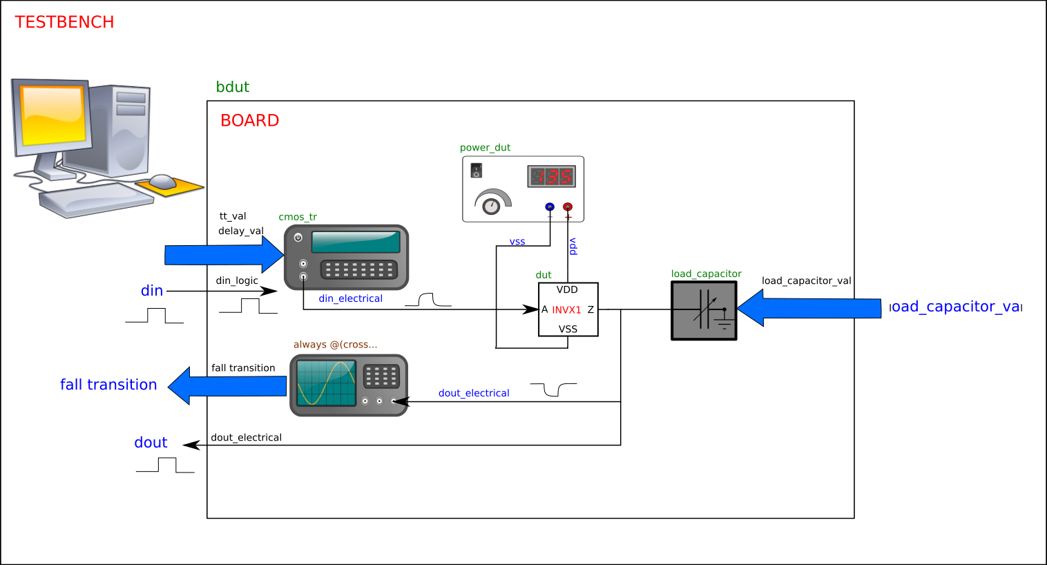
We organize the simulation in order to mimic the behavior of a physical system of data generation and measurement acquisition. The simulation code is splitted into 3 levels:

• The so-called “testbench” level, for the generation of digital input waveforms, the generation of several values of input parameters and for extraction of the measured results. (SystemVerilog).

• The so-called “board” level for the  power supplies, generators, analyzers (Verilog-AMS) connected to the device under test.

• The so-called “dut” level (dut means “Device Under Test, here the netlist of the cell to characterize) (Verilog-AMS)

Characterization

1. Download and extract the INVX1_fall_transition.tar.gz archive into your working directory. You should have now a new directory named INVX1_fall_transitioni.

2. Open a terminal, and get inside the new directory.   Inside this directory, several files needed for simulation of a INVX1 invertor from the standard cell library are present.  The following table explain the usage of this files. The main files (those file that you will have to modify through the project are written in bold letters).

BEWARE: You may access to informations about the languages and tools used, but it is not in the scope of this training module to learn all about these languages. During the project, you just have to understand the example codes, and adapt theses codes to your needs.

Filename	Usage
Makefile	All processings will be done via this Makefile. If you simply launch “make” you will have a  help message with list of all possible commands. For example, if you want to perform simulation, just launch “make simulation”.  For informations about makefiles, see here.
board.vams	The Verilog-AMS code describing the “board”. For informations about Verilog-ams, see here.
testbench.sv	The SytemVerilog code describing the “testbench” For informations about SystemVerilog, see here.
cmos_transition.vams	A Verilog-AMS module used to generate realistic CMOS electrical transitions from digital  transitions (0->1, or 1->0)
amsIrunControl.scs	A minimalist Spectre control file used by “Cadence irun” tool for mixed mode simulation
probes.tcl	Definition of the probed signals for eventual waveform display. All digital waveforms are probed, all electrical voltages are probed. Alls current through the ports of the device under test are probed
plot.py	A python script used to genrate curves from the measured datas.

3. Run  ”make” inside the simulation directory.  You should see the following help message:

simu          : simulation
show_waves    : examine simulation waveforms
plot_results  : examine simulation results
clean         : cleaning of the simulation directory, yet keeping last results
ultraclean    : cleaning of the simulation directory, removing all results
template_dir  : create a template dir for a new chararecterization job

 This message explains that the “make” command my be launched using six options. The detail usage of these options are in the following table:

Command	Usage
make simu	Launch the simulation. This is a non-interactive simulation. You should only see information, warning and error messages.
make show_waves	Launch a graphic tool in order to examine all digital and analog signal.  You should use this tool in order to check “sanity” of you simulation, or examine some internal signals
make plot_results	Launch a python script in order to display the extracted results in a graphic way
make clean	Clean the directory from temporary files, keeping the final results
make ultraclean	Clean the directory keeping only the source codes.
make template_dir	Create a template directory, with all needed source code, in order to prepare a new characterization simulation, while keeping the current code.

4. Run  ”make simu”:

• A new sub-directory named “results” should have been created.

• Inside the directory, you should find a file named “INVX1_fall_transition.dat”.

• This file contains the results of the characterization.

• Each line contains results for a selected rise time (i_slope)  of the input of the invertor.

• Each result is a pair with, a load capacitance (ldcap) and a fall transition time (o_fall).

• This file may be imported in any analysis tools of your choice  (spreadsheet or plot program).

BEWARE: When performing characterization do not trust obtained results. You should always check the extracted values and ask if they are realistic. In case of doubt, check the warnings or errors of the simulation phase, and check the waveforms.

5. Run  ”make show_waves”.

The “Viva” cadence waveform viewer is launched using the waveform database of you simulation.

• Open the hierarchy in the browser sub-window up to the “testbench” folder.

You should see signals known at the level of the testbench model. Signals flagged with “L” are purely binary signals of the testbench.

• Select the “din” , and “dout” signals. With the right button select “Plot signal”.

You should see the 2 waveforms. (dont worry the colors…)

• Signal flagged with “R” are real values used to transmit parameters from and to the testbench. Display the “tt_val” and “load_capacitor” val. In the graphic window, separate the two signals into two separate sub-windows.

Theses values are generated by the testbench to the board and used by the board to change the input transition of the invertor as well as the load capacitor.

• Open the hierarchy up to the “bdut” level (the board) .  Electrical nodes are flagged by “V” (for voltages).

You may display the “din_electrical” and “dout_electrical” signal: the real electrical signals at the input and the output of the INVERTOR.

• Zoom around any transition in order to see realistic signals around the invertor.

6. Run “make plot_results”.

The python script “plot.py” is launched to display results using meaningfull curves. You may once-again check if the results are realistic, and save the curves if you want to put this results in a report.

7. Now, take time to examine the two files board.vams and testbench.sv in order to understand:

• The exact role of the testbench.sv code

• The exact role of the board.vams code

• You will have to modify this files according to the kind of simulation you want to do…, but we will not ask you to learn all of the languages.