Rossler:
We consider the so-called Rössler prototype-4 system given by (see [2]):
\begin{cases}
\overset{.}{x} = -y -z\\
\overset{.}{y} = x\\
\overset{.}{z} = -b z + a(y-y^2)\\
\end{cases}
where \((x, y, z) \in \mathbb{R}^3\) are the state variables. Originally, Rössler in [1] has proposed a few abstract three-component chemical models (systems) which have chaotic solutions.
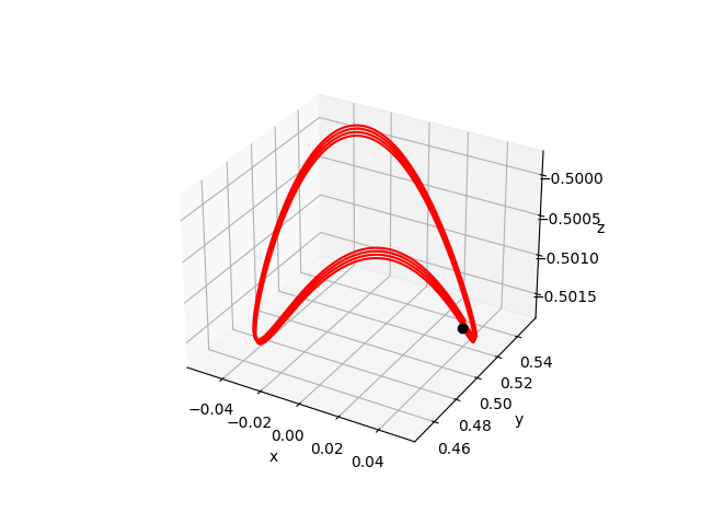
We consider the parameter values \(a = -1.51, b = 0.75\) and initial condition
\(X(0) = (0.04913235693166898, 0.5012738092954635, -0.5012724341616831) \).
Results:
We consider a system with uncertainty \(w=0.01\), set of initial conditions \(B(X_0,\varepsilon)\) with \(\varepsilon=0.05\), the time-step used in Euler's method is \(\tau = 10^{-4}\), and we take \(T=k\tau\) with \(k=62804\) as an approximate period.
For this example, we check that:
- \(B((i_0+1)T)\subset B(i_0T)\) for \(i_0=0\)
- and \(\Sigma_{i=1}^k\lambda_i\approx\) \(-23623< 0\).
Then, we can conclude that the system
converges towards an attractive LC
contained in
\([B(0),B(T)]\).
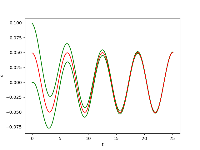
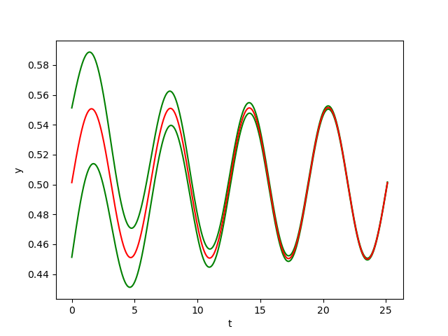
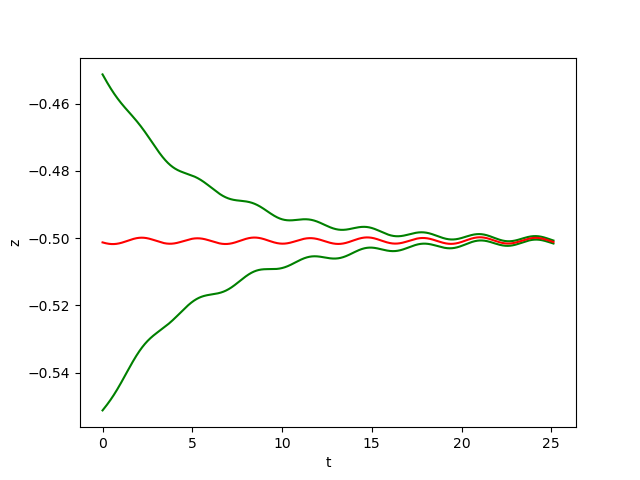
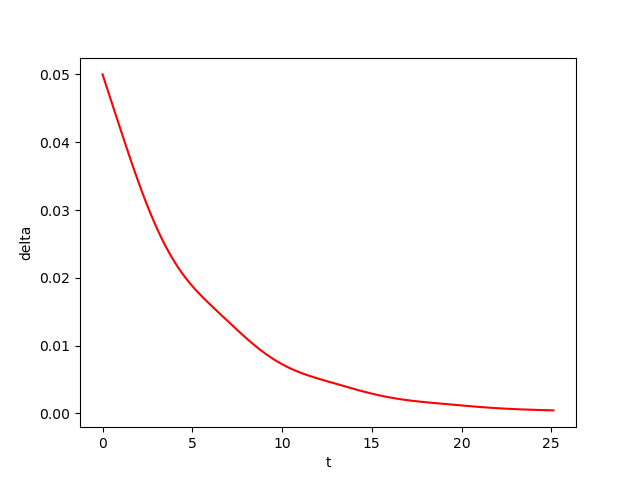
The figures below show respectively the simulation of \(x(t), y(t), z(t)\) and \(\delta_{{\cal W}}(t)\) with perturbation (w=0.01) over 4 periods (4T=25.1217) for dt=0.0001.
In the figrues \(x(t)\), \(y(t)\) and \(z(t)\), the red curves represent the Euler approximation and the green curves correspond to the borders of tube \(B\)
References:
[1] Rössler, O. Chaos and strange attractors in chemical kinetics. Springer Ser. Synerg. 1979, 3, 107–113.
[2] NIKOLOV, Svetoslav G. and VASSILEV, Vassil M. Dynamics of Rössler Prototype-4 System: Analytical and Numerical Investigation. Mathematics, 2021, vol. 9, no 4, p. 352.