Van der Pol:
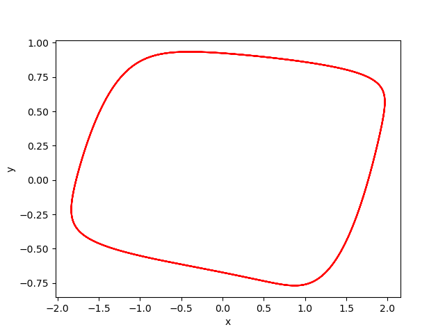
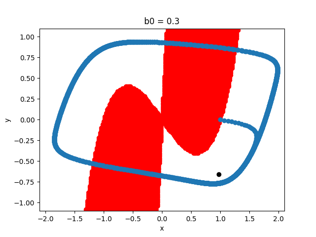
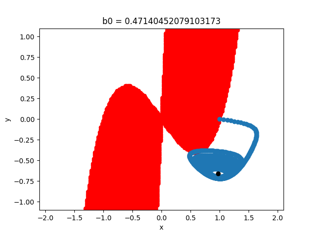
We consider Van Der Pol system [1] with: \begin{equation*} \begin{cases} \overset{.}{x}(t) = 10 (y + x - 1/3 x^3)\\ \overset{.}{y}(t) = b_0 - x - 0.75y \end{cases} \end{equation*} We present below some simulations of \(y(x(t))\) first with \(b_0=0.3\) and then with \(b_0=\sqrt(2)/3\). In the two cases, the blue curve designates the simulations of \(y(x(t))\), the red zone indicates the expansive area (\(\lambda>0\)) and the black point shows the fixed point at the saddle-node bifurcation. In the first figure (when \(b_0=0.3\)), x and y form a limit cycle. In the second figure (when \(b_0=\sqrt(2)/3\approx0.471\) at the saddle‐node (SN) bifurcation), the limit cycle collides with the fixed black point \(\approx (0.97,-0.66)\) and disappears.
Results:
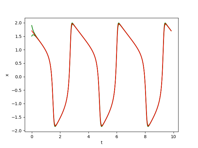
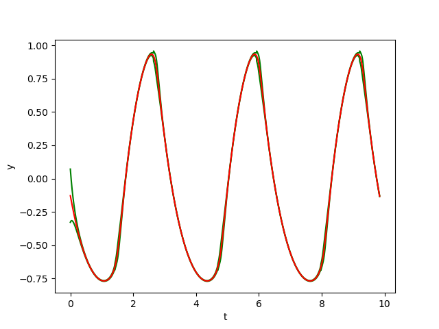
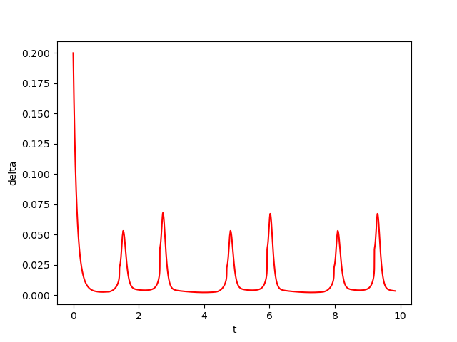
The figures below show respectively the simulation of \(x(t), y(t), y(x)\) and \(\delta(t)\) with perturbation (\(w=0.01\)) over 3 periods (\(3T=9.84\)) for \(dt=10^{-3}\) with initial conditions \((x(0), y(0)) = (1.70177925, -0.128415)\) and \(B(X_0,\varepsilon)\) with \(\varepsilon=0.2\) (See [2]). In the figrues \(x(t)\) and \(y(t)\), the red curves represent the Euler approximation, the green curves correspond to the borders of tube Bw.
For this example, we check that:- \(B((i_0+1)T)\subset B(i_0T)\) for \(i_0=2\)
- and \(\Sigma_{i=1}^k\lambda_i\approx\) \(-36065< 0\).
To get more results and details, Click Here