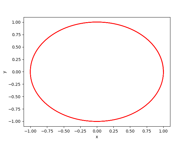
Hopf oscillator:
We consider the Hopf oscillator, the differential equations of the system are given below (See [1]):
\begin{cases}
\overset{.}{x} = (\mu - (x^2+y^2))x - \omega y \\
\overset{.}{y} = (\mu - (x^2+y^2))x + \omega x
\end{cases}
where \((x, y) \in \mathbb{R}^2\) are the state variables.
We consider the parameter values \(\mu = 1, \omega = 10\) and initial condition
\(x(0) = (1, 0) \)
Results:
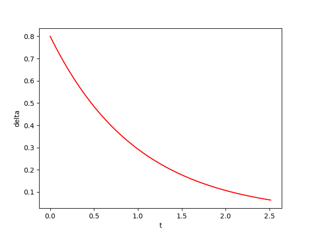
We consider a system with uncertainty \(w=0.1\), set of initial conditions \(B(x_0,\varepsilon)\) with \(\varepsilon=0.8\), the time-step used in Euler's method is \(\tau = 10^{-4}\), and we take \(T=k\tau\) with \(k=6284\) as an approximate period.
Using the figures shown below, we check that:
- \(B((i_0+1)T)\subset B(i_0T)\) for \(i_0=0\)
- and \(\Sigma_{i=1}^k\lambda_i\approx\) \(-12657< 0\).
Then, we can conclude that the system
converges towards an attractive LC
contained in
\([B(0),B(T)]\).
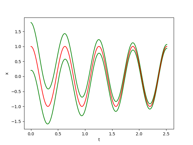
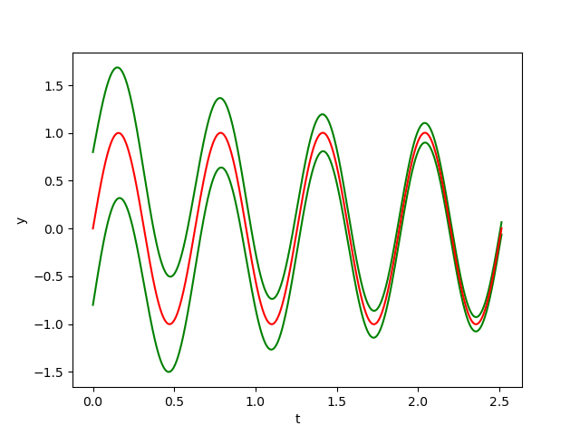
The figures below show respectively the simulation of \(x(t), y(t)\) and \(\delta_{{\cal W}}(t)\) with perturbation (w=0.1) over 4 periods (4T=2.5137) for dt=0.0001.
In the figrues \(x(t)\) and \(y(t)\), the red curves represent the Euler approximation and the green curves correspond to the borders of tube \(B\)
References:
[1] RIGHETTI, Ludovic, BUCHLI, Jonas, and IJSPEERT, Auke Jan. Dynamic hebbian learning in adaptive frequency oscillators. Physica D: Nonlinear Phenomena, 2006, vol. 216, no 2, p. 269-281.