ORBITADOR

Gradient Descent with Periodic Entrainement on the Loss Surface of Neural Networks:

Consider the entrained system with initial condition \(y_0\) (see [1]): \begin{equation}\label{eq:GDE0} \dot{y}(t)=g(y(t))+\gamma(t)\varphi(t) \end{equation} with \(g:\mathbb{R}^p\rightarrow\mathbb{R}^p\), \(y(0)=y_0\in\mathbb{R}^p\) and \(\gamma(t)=\alpha\beta(t)\) where

• \(\alpha\in\mathbb{R}_{\geq 0}\) is the amplitude factor,
• \(\beta:\mathbb{R}_{\geq 0}\rightarrow [0,1]\) the slow periodic function with period \(U\),
• \(\varphi:\mathbb{R}_{\geq 0}\rightarrow [-1,1]^p\) the fast periodic function with period \(T\)

We consider now a NN where the second layer is fixed and GD is applied on the first layer weights matrix (see [2, 3]). \begin{equation}\label{eqn:layer2} \tilde{w}_{k+1}=\tilde{w}_k-h \frac{\partial {\cal L}(\tilde{w}_k)}{\partial w_k} +h\gamma(hk) \varphi(hk) \end{equation} where the gradient formula for each weight vector is \begin{equation*} \frac{\partial {\cal L}(w)}{\partial w^r}=\frac{1}{\sqrt{m}}\sum_{i=1}^nv^ia_r x_i \textcolor{blue}{\mathbb{I}}\{x_i^\top w^r\geq 0\}. \end{equation*} with \(r\in \{1,\dots,m\}\) and \(\textcolor{blue}{\mathbb{I}}\) is the indicator.
\(v(t)=(v^1(t),\dots,v^n(t))\in\mathbb{R}^{d\times n}\) is the error function: \begin{equation*} v^i(t)=f(w(t),a,x_i)-y_i\in\mathbb{R}^d. \end{equation*} where \( f \) is a NN of the form: \begin{equation} f(w,a,x)=\frac{1}{\sqrt{m}}\sum_{r=1}^ma_r \sigma(x^\top w^r) \end{equation} \(x\in\mathbb{R}^d\) is the input, \(w=(w^1,\dots,w^m)\in\mathbb{R}^{d\times m}\) is the weight vector of the first layer, \(a_r\in\mathbb{R}\) is the output weight and \(\sigma(\cdot)\) is the ReLU activation function: \(\sigma(z)=z\) if \(z\geq 0\) and \(\sigma(z)=0\) if \(z<0\).

To get the code source: Click Here

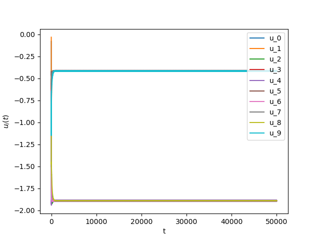
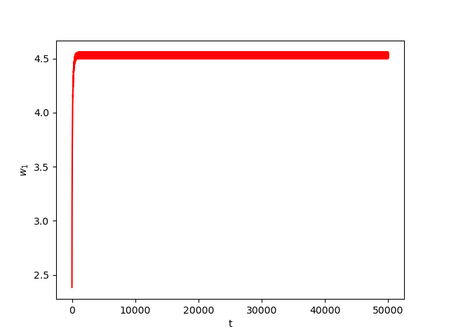
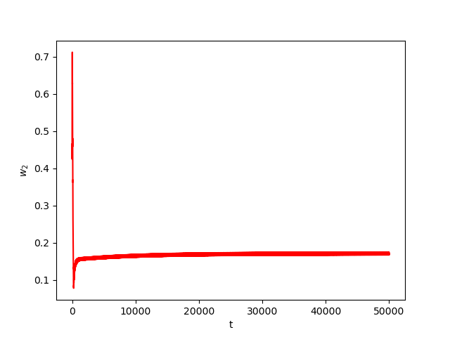
Numerical Example 1:

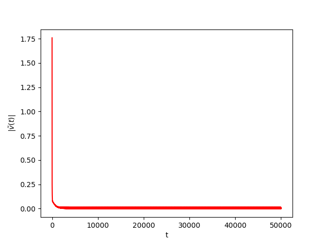
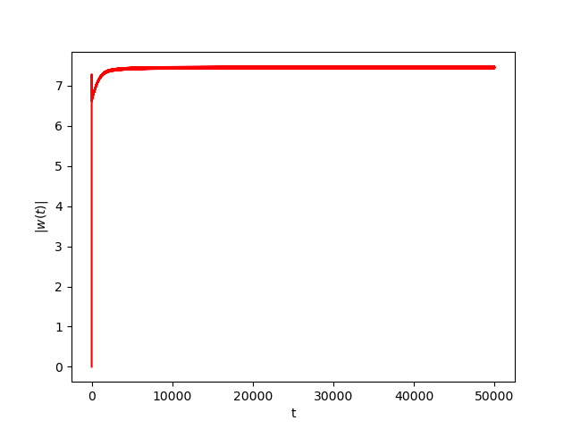
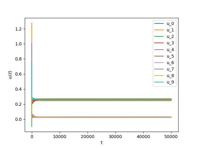
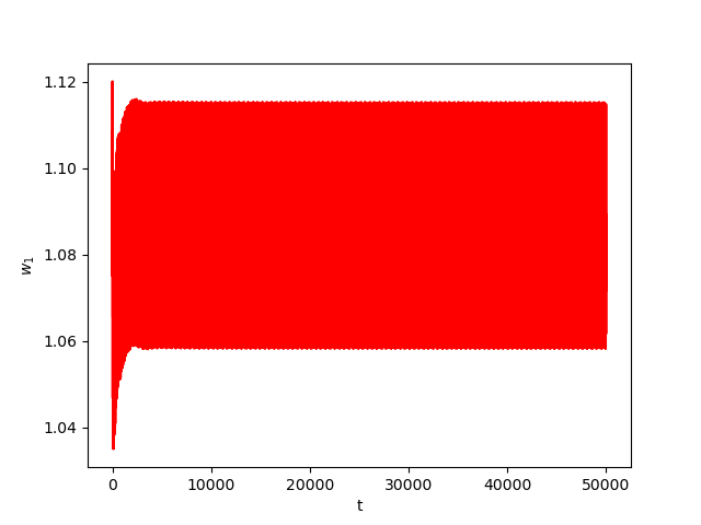
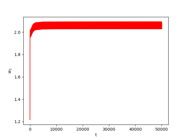
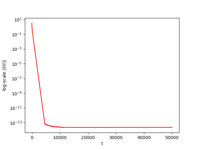
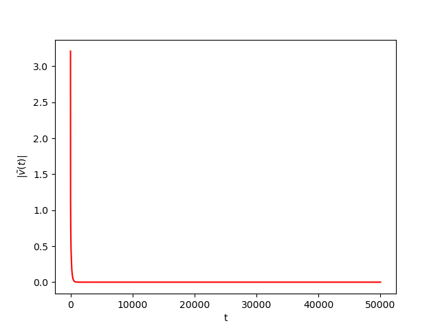
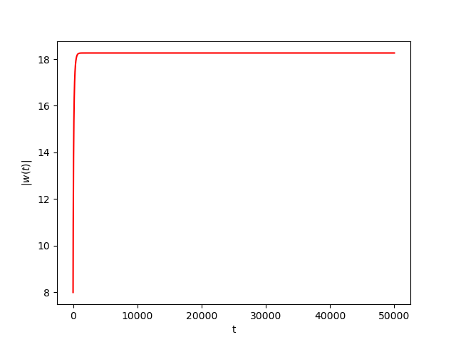
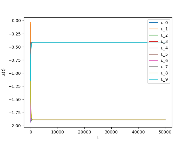
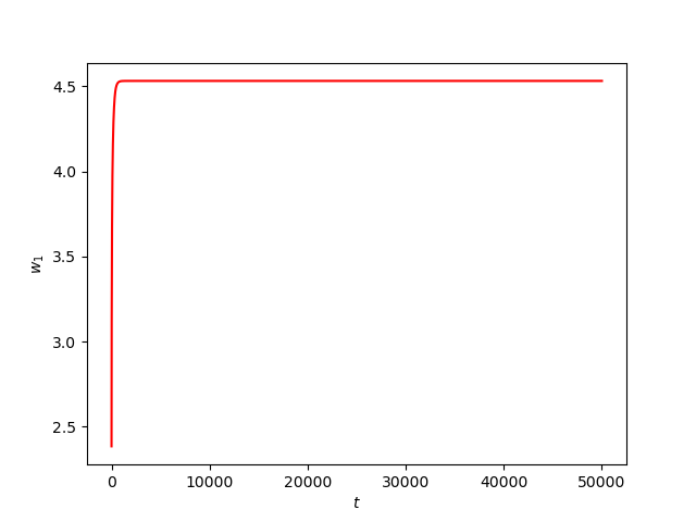
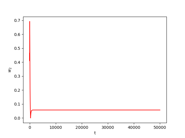
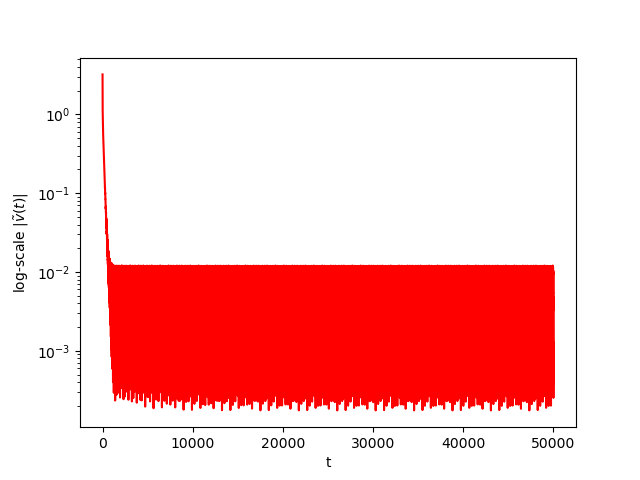
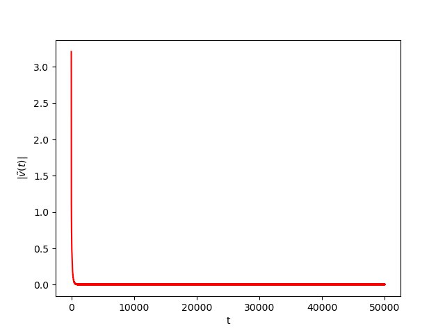
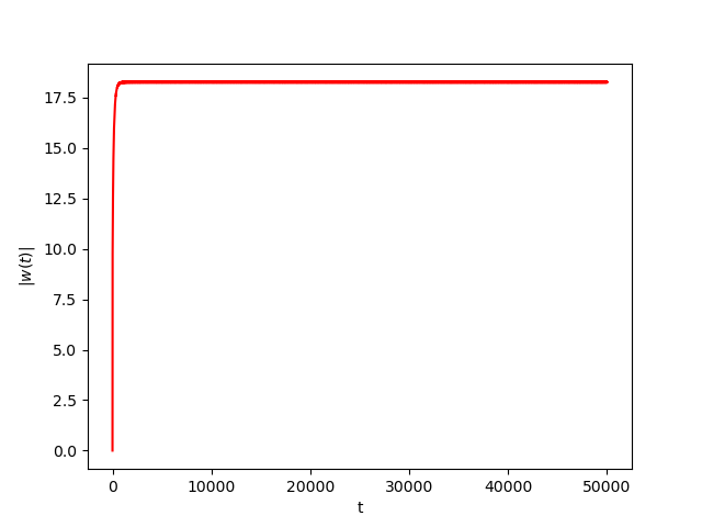
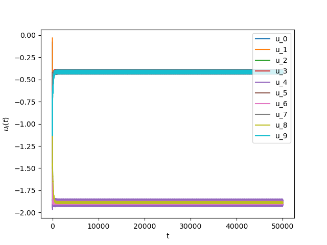
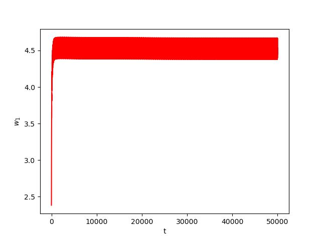
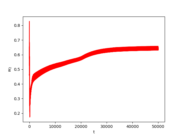
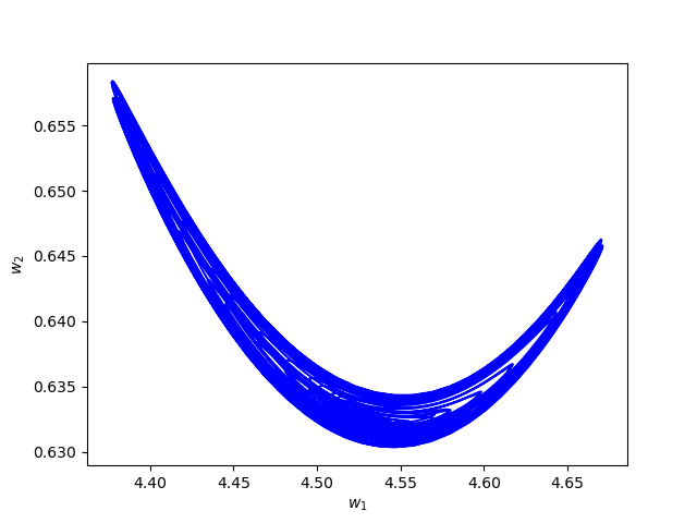
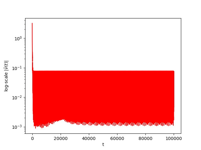
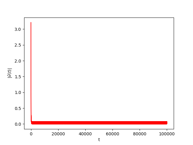
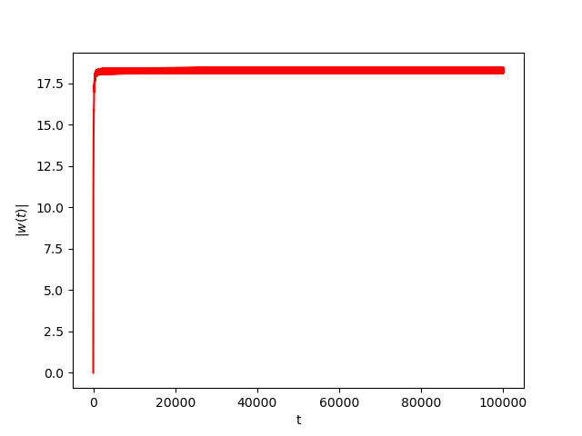
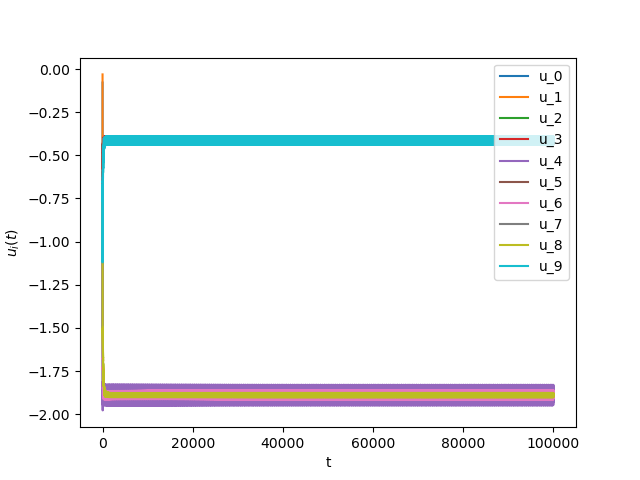
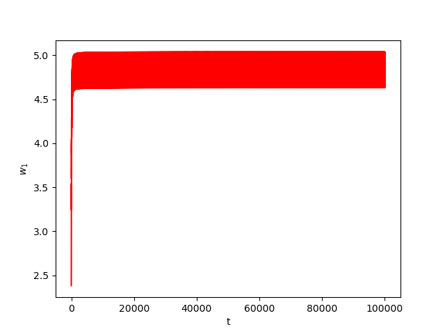
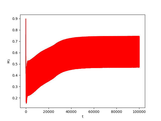
We consider The training has been conducted using \(n=10\) data points, \(m=20\) hidden nodes and \(d=3\). We take \(h=0.15\), \(\varphi=\cos(\frac{t}{2})\) and \(\alpha=0\). The initial conditions and the initial first layer weight vector \(w^r\) are picked randomly.

Results:

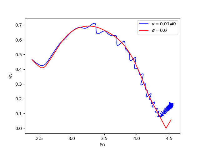
Numerical Example 2:

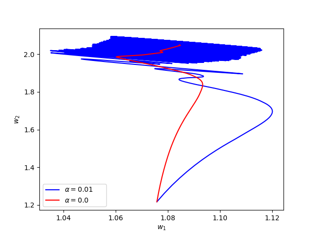
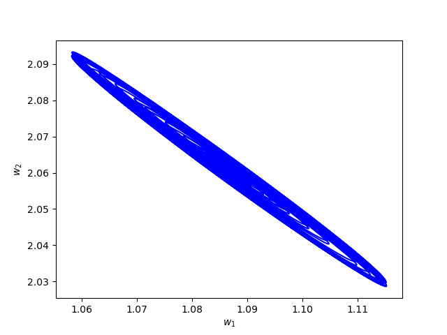
Now we consider the same example but with \(\alpha=0.01\) and \(\beta(t)\in [0,1]\) is a triangular signal of period \(U=2.5T=10\pi\).

Results:

Numerical Example 3:

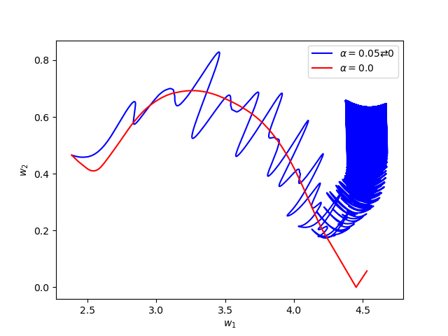
Now we consider the same example but with \(\alpha=0.05\) and \(\beta(t)\in [0,1]\) is a triangular signal of period \(U=2.5T=10\pi\).

Results:

Numerical Example 4:

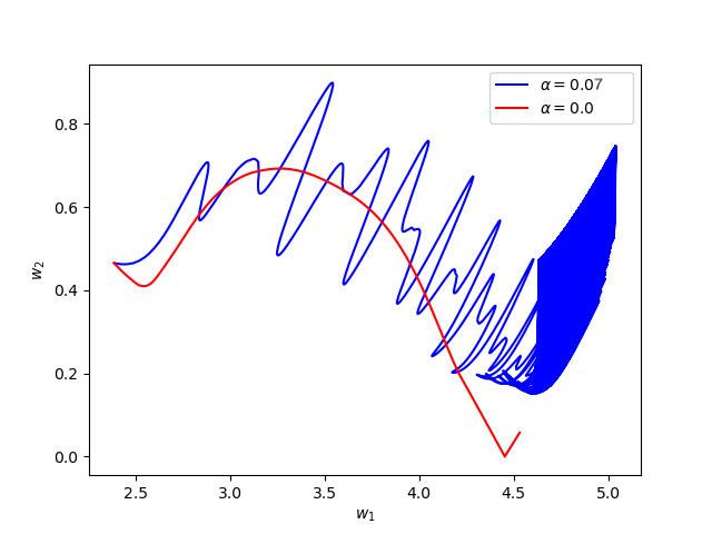
Now we consider the same example but with \(\alpha=0.07\) and \(\beta(t)\in [0,1]\) is a triangular signal of period \(U=2.5T=10\pi\).

Results:

Numerical Example 5:

We consider the same example but with differant inital conditions, \(\alpha=0.01\) and \(\beta(t)\in [0,1]\) is a triangular signal of period \(U=2.5T=10\pi\).

Results: