Brusselator:
We consider the 1D Brusselator partial differential equation (PDE)[1].
Here we consider a state of the form \(x(y,t)=(u(y,t),v(y,t))\)
where \(y\in \Omega = [0,\ell]\) is the spatial location. The PDE is of the form:
\begin{cases}
\frac{\partial u}{\partial t} = A+u^2v-(B+1)u+\sigma \nabla^2 u\\
\frac{\partial v}{\partial t} = Bu-u^2v+\sigma \nabla^2 v
\end{cases}
with boundary condition:
\(u(0,t)=u(\ell,t)=1\), \(v(0,t)=v(\ell,t)=3\)
and initial condition \(x_0(y)=(u(y,0),v(y,0))\) with:
\(u(y,0)=1+sin(2\pi y)\), \(v(y,0)=3\).
We consider: \(A=1, B=3, \sigma=1/2\), \(\ell =1\).
We transform the PDE into a system of ODEs
by spatial discretization using
a grid of \(N+1\) points with \(N=4\) (See [2]).
We thus consider that we have \(4\) oscillators
of state \(x(y_i,t)\equiv (u(y_i,t),v(y_i,t))\)
with initial conditions \(x(y_i,0)\equiv (u(y_i,0),v(y_i,0))\) (\(i=1,2,3,4\)).
The system of ordinary differential equations for this example is described by:
\begin{equation}
\begin{cases}
\overset{.}{u_1} = A+u_1^2v_1-(B+1)u_1+\sigma (u_0 - 2u_1 + u_2)\\
\overset{.}{v_1} = Bu_1-u_1^2v_1+\sigma (v_0 - 2v_1 + v_2)\\
\overset{.}{u_2} = A+u_2^2v_2-(B+1)u_2+\sigma (u_1 - 2u_2 + u_3)\\
\overset{.}{v_2} = Bu_2-u_2^2v_2+\sigma (v_1 - 2v_2 + v_3)\\
\overset{.}{u_3} = A+u_3^2v_3-(B+1)u_3+\sigma (u_2 - 2u_3 + u_4)\\
\overset{.}{v_3} = Bu_3-u_3^2v_3+\sigma (v_2 - 2v_3 + v_4)\\
\overset{.}{u_4} = A+u_4^2v_4-(B+1)u_4+\sigma (u_3 - 2u_4 + u_5)\\
\overset{.}{v_4} = Bu_4-u_4^2v_4+\sigma (v_3 - 2v_4 + v_5)
\end{cases}
\end{equation}
with \(u_0=u_5=1\) and \(v_0=v_5=3\).
Results:
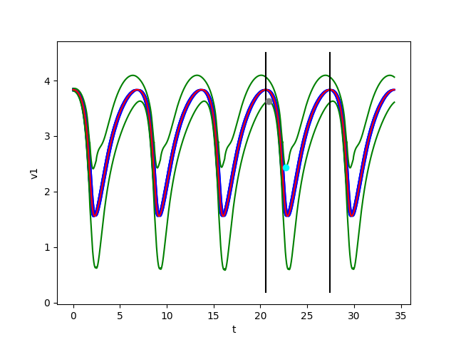
We consider a system with uncertainty \(w\in {\cal W}=[-0.05,0.05]\), set of initial conditions \(B(x_0,\varepsilon)\) with \(\varepsilon=0.02\), the time-step used in Euler's method is \(\tau =2\cdot 10^{-4}\), and we take \(T=k\tau\) with \(k=34302\) as an approximate period.
Using the figures shown below, we check that:
- \(B((i_0+1)T)\subset B(i_0T)\) for \(i_0=3\)
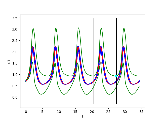
- also for \(u_1\), the minimum \(m^1_+= 0.92679\) (represented by a small cyan ball) of the upper green curve \(\tilde{u}_1(t)+\delta_{{\cal W}}(t)\) is less than the maximum \(M^1_-= 1.51263\) (represented by a small gray ball)
of the lower green curve \(\tilde{u}_1(t)-\delta_{{\cal W}}(t)\)
- and \(\Sigma_{i=1}^k\lambda_i\approx\) \(-27147.716 < 0\).
Then, we can conclude that the system
converges towards an attractive LC
contained in
\([B(3T),B(4T)]\).
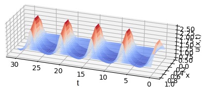
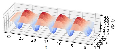
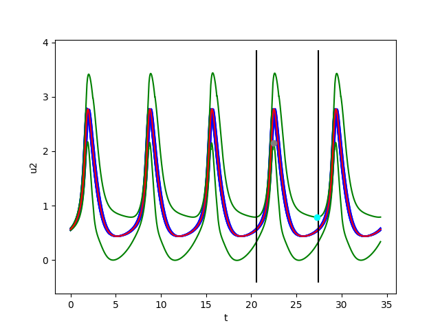
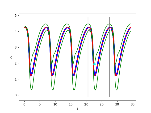
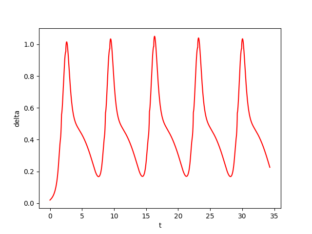
The figures below show respectively the simulation of \(u_1(t), u_2(t), v_1(t), v_2(t)\) and \(\delta_{{\cal W}}(t)\) with perturbation (w=0.05) over 5 periods (5T=34,3) for dt=0.0002. The red curves represent the Euler approximation, the green curves correspond to the borders of tube \(B_w\).
The black vertical lines delimit the portion of the tube between \(t=i_0*T_0\) and \(t=(i0+1)T_0\). The cyan point represents the minimum \(m_+^1\) of the upper green curve and the gray point shows the maximum \(M_-^1\) of the lower green curve.
To get more results and details, Click Here
References:
[1] CHARTIER, Philippe and PHILIPPE, Bernard. A parallel shooting technique for solving dissipative ODE's. Computing, 1993, vol. 51, no 3-4, p. 209-236..
[2] JERRAY, Jawher, FRIBOURG, Laurent, and ANDRÉ, Étienne. Guaranteed phase synchronization of hybrid oscillators using symbolic Euler's method (verification challenge). EPiC Series in Computing, 2020, vol. 74, p. 197-208.