Objectives
The goal of this lab is to provide a gentle introduction to D3, one of the environments we will use for this class. It will also help you get used to drawing to the screen, loading data from a file, and thinking about how to represent data.
What is D3?
D3 is a JavaScript library for creating Data-Driven Documents on the web. It uses a complex model that simplifies many of the tasks of creating visualizations on the web. In order to use it, you will need to understand:
- JavaScript
- The HTML Document Object Model (DOM)
- The SVG vector graphics format
- Cascading Style Sheets (CSS)
In this lab, we will provide a brief introduction to these concepts so that we can create a basic visualization. There is also a Python version and a Java version of this lab available using the Processing environment, which is less well-known than D3 but has a strong community and has been used to create numerous visualizations. If you feel overwhelmed by the complexity of D3, Processing is a great tool to add to your toolbox.
Getting started
You create a D3 visualization using any standard programming environment for web documents. You can use your own preferred environment for web development (e.g. TextMate, Sublime Text, vi, emacs, …), just make sure it has proper support for web development. If you’re not sure, here’s a link to Microsoft’s Visual Code editor. And here are some locally cached copies for Mac, Windows. (There’s a Linux version, too, but I couldn’t download it from my Mac.)
Part 1
In our first project, we are going to learn how to use D3 to create the following image:
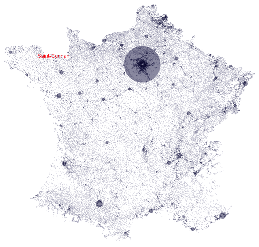
In order to do so, you will need to:
- Load and parse the data.
- Choose an internal data structure to represent these data.
- Draw them to the screen.
The data we will use comes from www.galichon.com/codesgeo. The original data was in the form:
- (name, postal code, insee code, longitude, latitude)
- (name, insee code, population, density)
To simplify things, we will instead use a pre-processed version of these data courtesy of Petra Isenberg, Jean-Daniel Fekete, Pierre Dragicevic and Frédéric Vernier. It merges these into:
- (postal code, x, y, insee code, place, population, density)
Getting started
First, let’s create a new folder for our project. Let’s call it France, and add three subfolders: css, js, and data. You should have a structure something like this:
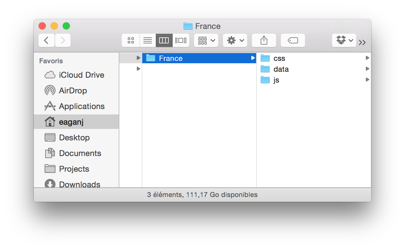
Next, open up your project in your favorite web programming editor. Notice that we have our three subfolders. The first thing we will need is a blank canvas to work with. In D3, our documents are “just” web pages. Create a new HTML document and add some boilerplate code for a basic HTML document.
In this lab, I’ll start off by showing you the code to write. As we progress, I’ll show you less and less, and leave more open to your own interpretation. Please resist the temptation to just copy and paste the code. It’s important to understand what’s going on. Even if it seems obvious, writing (or typing) the code out by hand helps to reinforce things in your mind, so please type the following code in the window:
:::html
<html>
<head>
    <meta charset="utf-8">
    <title>Hello, France (D3)</title>
</head>
<body>
</body>
</html>
Let’s save this file as index.html, the default web document that browsers will see when they open our project. This gives us a blank web page with the title Hello, France (D3). Let’s make sure by opening it in our web browser. (In case you’re wondering about the <meta charset> line, that tells the web browser that our HTML uses UTF-8 text encoding, which helps make sure that our French accents will appear correctly on the screen.)
This blank document is awfully boring, so let’s get ready to start adding some content to it. In D3, we will be adding our content programmatically, using JavaScript. To that, let’s add the D3 library to our project. Download the D3 library and extract it into the js/ folder in our project. Our project should now look like this:
- France
- css/
- data/
- index.html
- js/
- d3
- d3.js
- d3.min.js
- LICENSE
- d3
Let’s tell our project to use the d3.js library. Add the following line to the HTML header section of our document:
:::html
<script type="text/javascript" src="js/d3/d3.js"></script>
And now we need to create a file where we’ll put our own code. Create a new file, save it as js/hello-france.js, and tell our project to load it by adding the following like to the HTML body section of our document:
:::html
<script type="text/javascript" src="js/hello-france.js"></script>
Let’s make sure everything is loading correctly. Add the following line to the hello-france.js document:
:::js
alert("Hello, France!");
When we load our page, we should see our message in an alert box. If not, make sure you’ve correctly added your <script> tag in your HTML body section or see if there’s anything else weird going on. Once everything is in order, let’s go ahead and remove the alert() call, since that will get annoying quickly.
Congratulations! You now have a blank skeleton of your project set up.
Creating an empty canvas
So far, we have an HTML document that loads D3 and our JavaScript code. We now need to create a drawing canvas we can use to create our visualization. To do that, we will use SVG, a vector graphics format that uses the same syntax as HTML. In fact, it is a superset of HTML and will be a part of our DOM. A blank SVG document, at its most simple, is just <svg></svg>. Let’s tell our hello-france.js to create a blank canvas for us, 600 pixels wide by 600 pixels high:
:::js
var w = 600;
var h = 600;

//Create SVG element
var svg = d3.select("body")
            .append("svg")
            .attr("width", w)
            .attr("height", h);
Let’s take a closer look at what this does. The first two lines should be straightforward: we create two global variables, w and h, that store the dimensions of our canvas. It’s the next part that is tricky. First, D3 creates a global variable, d3, that we will use to interact with the D3 system.
D3 uses a notion of selectors similar to that of jQuery. As such, when we write d3.select("body"), d3 will traverse the DOM and return all of matching elements. In this case, all <body> elements. Our document (and any proper HTML document) only has one.
The next line, .append("svg"), appends a new <svg></svg> element as a child of the resulting <body> element. Thus, a document with an empty body:
:::html
<body></body>
would become:
:::html
<body>
    <svg></svg>
</body>
The result of the .append() method is the newly added SVG element, to which we then set it’s “width” attribute to w (600) using the attr() method. D3 uses a “chaining” model for its methods, where methods that would otherwise be void instead return their object. Thus, the result of this .attr() is the SVG element whose attributes we are setting.
At the end of this, our document now looks like:
:::html
<body>
    <svg width="600" height="600"></svg>
</body>
If you look at your index.html file, you might think this is crazy, since it has not changed. There are no new lines in the file. Remember: in D3, we are programmatically modifying the DOM. When the web browser loads our document, it will create it’s internal model of the document (the DOM) using what was in the .html file. From then on, our JavaScript modifies this internal document. It is entirely ephemeral: it does not modify the .html file on disk.
Loading data
Now lets take a look at the data we’re going to use. Open them in your preferred text editor or in your favorite spreadsheet program. Notice that this a file containing a data table in a tab-separated format. What are the attributes of the data file? Do you notice anything interesting about the data?
The first thing we need to decide is how to store our data. Generally D3 stores data as a list of values. Here, each value will be a row in our table, which we will store as a JavaScript dictionary, or object. Each entry should have a postal code, INSEE code, place name, longitude, latitude, population, and population density. We will need to define a loader that will fetch each row of our TSV file and convert it into a JavaScript object.
Let’s go ahead and read the data into D3. D3 provides various importers to handle data in different formats, such as csv, tsv, json, etc. For more information, take a look at the D3 API. Since our data consists of tab-separated values, we are going to use the tsv loader.
D3 loaders generally return immediately so that the interface can continue to run before all of the data has been loaded. We need to pass it a function that will be called for each row as it is loaded. That function is named, surprisingly enough: row().
:::js
d3.tsv("data/france.tsv")
    .row(function (d, i) {
        return {
            codePostal: d["Postal Code"],
            inseeCode: d.inseecode,
            place: d.place,
            longitude: d.x,
            latitude: d.y,
            population: d.population,
            densite: d.density
        };
    })
Let’s take a closer look at what that does. First, we use d3.tsv() to asynchronously load our data from the specified URL (data/france.tsv). Next, we use the .row() method to set the function that will be called for each row in the TSV file. We pass it one parameter: a function (which we define here) that takes two parameters:
d, a JavaScript dictionary whose keys are the column labels from our TSV file, andi, the index of the current row.
Notice that the first column has a space in its name, and is thus not a valid JavaScript attribute name. We therefore need to access it using dictionary notation: d["Postal Code"]. The others are valid attribute names, so we can just access them as attributes, as in d.place.
If we leave our code as is, nothing will happen. So far, we have told D3 what file we want to load and how to handle each row, but we have not yet told it to actually load the data. We do that with the .get() method. Here, too, we need to pass in a function. This function will be called when the file has finished loading. It takes two parameters: an error parameter that will be set if an error occurs, and the list of rows, generated by our .row() function above.
:::js
    .get(function(error, rows) {
        console.log("Loaded " + rows.length + " rows");
        if (rows.length > 0) {
            console.log("First row: ", rows[0])
            console.log("Last  row: ", rows[rows.length-1])
        }
    });
Here, we just output some debugging information to the console, so we can make sure everything is loading correctly. Take a look at the first and last rows. Maybe try with a few random rows, too, just to do a spot-check. Does everything look right?
Converting the data
So far, everything looks pretty good, but you might have noticed a problem at the end of the last section. If we take a closer look at our console log, we should see something like this:
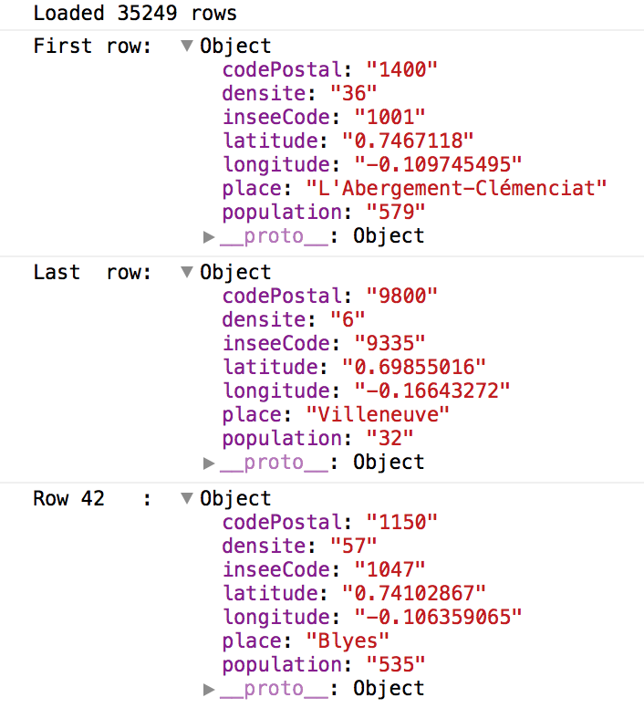
Do you see the problem?
It’s subtle, but it’s there.
Try to see if you can figure it out before you read on.
Did you figure it out?
Yes, that’s right, all of our values are strings, including numerical attributes such as population, longitude, and latitude. Thankfully, there’s a concise way to convert these strings to numerical values in JavaScript: use the + operator. Modify your .row() method above to replace all of the numerical attributes as follows such that, for example, d["Postal Code"] becomes +d["Postal Code"].
Try reloading the page in your browser and make sure you see the right thing on the console.
Drawing
Great, we now have a way to get data into our document. So far, it doesn’t really do us much good if we can’t somehow draw it to the screen. Let’s figure out how to do that.
First, we’re going to need to make sure we save the data somewhere we can use it. The rows parameter to our get() method has the data, so we just need to save it somewhere accessible from the rest of our program. Add a new global variable, just after your w and h variables, to store the dataset. Let’s call it dataset:
:::js
var w = 600;
var h = 600;
var dataset = [];
Now, at the end of the .get() method, store our rows in this variable: dataset = rows;. Then add a call to draw(), which we’ll define shortly. That way, once all of the data has been loaded, we will call draw() to draw all the data.
Enter, update, exit
Now we get to the hardest part of D3: enter, update, exit. D3’s data model takes some getting used to. What we’re really doing is defining rules that will be executed whenever our data changes in some way:
enterwhenever a new data entry is created,updatewhen a value changes, andexitwhen a value is deleted.
Each of these rules will tell D3 what to do, such as creating or removing a (new) element on our canvas or updating certain attributes of our elements.
In this example, our data set is not going to change, so we only need to use enter. For dynamic data sets, where entries may be created or removed while the page is being shown, or where entries may change values, you will need to use update and exit as well.
Let’s just create a small rectangle for each place in our data set:
:::js
function draw() {
    svg.selectAll("rect")
        .data(dataset)
        .enter()
        .append("rect")
}
So far, this function won’t actually draw anything, because we have not yet told it how to connect our rectangles to the data. We’ll do that shortly, but first let’s try to understand what’s going on above, since it’s a bit strange.
First, we use the svg variable we created earlier, which represents our canvas. We tell it to select all of the <rect>s in our drawing, then tell it to bind them to the data we stored in our dataset variable. We then use .enter() to specify that, when new data comes in (such as when we first load the document), it should append a new <rect> element to our canvas.
If your brain is having a hard time digesting this, that’s ok. It feels like we’re eating our cake before we bake it. First, we select all of the rects, then we create them. This is where we need to remember that what we are doing is defining a set of rules that will be used. Thus, we are not actually selecting all of the rects in the svg canvas. Instead, we are defining a rule that will be applied to all rects. When a new entry is created in our dataset, the rules we specify here after .enter() will be applied to them, which in this case is to create a <rect>, which is how SVG describes rectangles.
When we create a new rectangle, we want, for now at least, it’s size to be 1 × 1 pixels. We do that by specifying SVG and CSS attributes for the rect:
:::js
function draw() {
    svg.selectAll("rect")
        .data(dataset)
        .enter()
        .append("rect")
        .attr("width", 1)
        .attr("height", 1)
        // ...
}
We also want its position to correspond to its longitude and latitude. That’s a little bit trickier. So far, the width and height have been constant (1), but the position will be a function of the data (it’s longitude and latitude). We need a way to specify a different value specific to each point.
In D3, we can do that by passing in a function as the value. The function takes a single value as a parameter: our data point. It returns the value that we want to use. Thus, we can replace the ellipsis in the above code with:
:::js
.attr("x", function(d) { return d.longitude })
.attr("y", function(d) { return d.latitude })
What do you expect to happen when you run the program? Try it out. Reload the page. What actually happens? Can you think of a reason why we don’t see anything on the screen?
Before you get too far trying to figure out why you don’t see France, take a closer look at the top, left of our document. It’s subtle, but we do have a bunch of rectangles being created. Try to think about what might be going on.
Still not sure? Let’s take a closer look at our data. Recall that each row is in the following format:
(postal code, x, y, insee code, place, population, density)
We only use the x and y columns. Think about it before continuing on.
Data scales
The x and y columns in the data set are expressed in longitude and latitude, not in terms of pixel coordinates on the screen. All of our coordinates correspond to a single pixel, which is being clipped to the top left of our canvas since all of France has a negative longitude.
We need to create a mapping from longitude, latitude to x, y-coordinates on the screen. Assuming a flat projection, the math is actually pretty simple. Since this kind of problem is very common, D3 has a builtin concept for this: scales. We can define scaling functions that will map a value from one coordinate space to another. Here, we just have a linear scaling function, so we can use D3’s linear scales:
d3.scale.linear()
To do so, we will need to create our x-scale and y-scale that will map a longitude, latitude onto our 600 × 600 pixel canvas. To do that, we need to set the scale’s domain and range, which correspond to the range of values that an input can take, and the range of values an output can take on.
We could take a look at our input and figure out our domain from the longitudes and latitudes of our data set, but instead we’ll compute it dynamically from the data set. That way, if some day we want to show places in the United States or China or Antarctica, our visualization would handle it without trouble. To do so, we use D3’s extent() function, which gives the extent of the data set: the range of a given column’s min and max values. We will store these scales in two global variables: x and y. Go ahead and add these to the top of our file.
Now modify our data loader to compute the scales when the data is finished loading:
:::js
x = d3.scale.linear()
                    .domain(d3.extent(rows, function(row) { return row.longitude; }))
                    .range([0, w]);

y = d3.scale.linear()
                    .domain(d3.extent(rows, function(row) { return row.latitude; }))
                    .range([0, h]);
These scales will take a value in a given domain and normalize it to the given range. Let’s modify our drawing loop to use them as follows:
:::js
.attr("x", function(d) { return x(d.longitude) })
.attr("y", function(d) { return y(d.latitude) })
Let’s try running the program one more time, and this time we should be able to marvel in the wonder of your beautiful drawing. Or fix any bugs and then marvel.
Graphics coordinates
Have you noticed something peculiar about our map of France?
In most graphics environments, the origin (0, 0) is located at the top, left of the canvas. Latitudes, on the other hand, start at the equator, which we tend to think of as being to the bottom of France. No worries, all we need to do is invert either our domain or our range in the above mapping function.
Make that change and re-run the program. Is Corsica at the top or the bottom? Do we indeed see the Finistère next to the Channel, or is it hanging out in the Mediterranean?
On your own…
That’s great for getting started, but what we’ve created so far is really only little more than an info vis “Hello, world” (or, more properly, “Hello, France!”).
To better understand our toolbox, let’s look at the D3 API reference. These are the builtin methods and functions of D3. There’s a lot to take a look at. You may also wish to learn more about CSS or SVG.
You should now have the tools you need to update your visualization to:
- Show population and density
You’re also going to make your visualisation interactive. When the user clicks on a place, draw its name and postal code. You will need the following tools to do so:
Text rendering
Tell D3 to add a new text item below your canvas that you will use to display the names of places as the user hovers over them.
User events
You can use D3’s .on() method to add callbacks for certain events, such as mouseover or mouseout when the user hovers or unhovers on an item. For example:
:::js
.on("mouseover", function(d) { /* ... */ })
 Assignment based on one by Petra Isenberg, Jean-Daniel Fekete, Pierre Dragicevic and Frédéric Vernier under a Creative Commons Attribution-ShareAlike 3.0 License.