
Webinaire Data&IA @ IMT - https://mintel.imt.fr/voir.php?id=5212
Vers un calcul de la pertinence
Jean-Louis Dessalles
www.dessalles.fr /slideshows

Télécom Paris
Vers un calcul de la pertinence
- ML: la pertinence distingue les données du bruit
- ML: est pertinent ce qui est digne d’être appris/mémorisé
- ML: un outlier n’est pas pertinent...
- ... ou est très pertinent en tant qu’anomalie

Vers un calcul de la pertinence
- XAI: une explication est pertinente si elle peut convaincre
- NLG: une intervention est pertinente si elle est appropriée

- IA: Par définition (selon A. Turing),
une machine intelligente
se doit d’être pertinente.
- → Un problème fondamental pour l’IA !
- → Un problème fondamental en science !
- → Le problème scientifique le plus fondamental !
Qu’y a-t-il de commun ?

- bruit
- data utiles
- outliers
- anomalies
- explication
- intelligence
Algorithmic Information Theory (AIT)

- L’information est ce qui reste
quand toute redondance est éliminée - L’information se mesure en bits
- L’information au sens de Shannon est une moyenne statistique sur des événements répétés.
- Elle ne convient pas pour mesurer la pertinence
Vers un calcul de la pertinence
- Pertinence & Machine Learning
- Pertinence & AIQ (artificial IQ)
- Pertinence des événements
Vers un calcul de la pertinence
- Pertinence & Machine Learning
- Pertinence & AIQ (artificial IQ)
- Pertinence des événements
Algorithmic Information Theory (AIT)
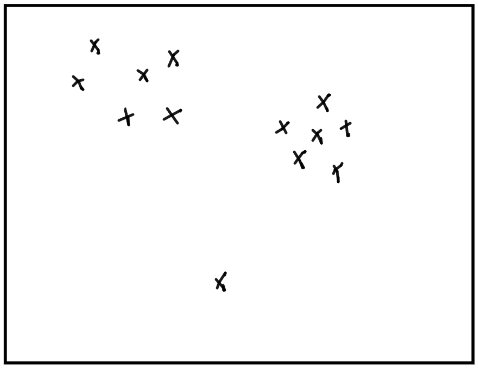 Représenter des données de manière pertinente.
Algorithmic Information Theory (AIT)
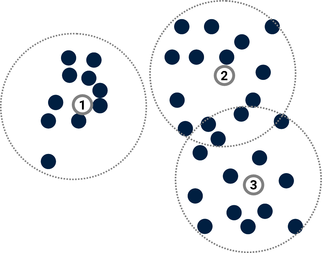
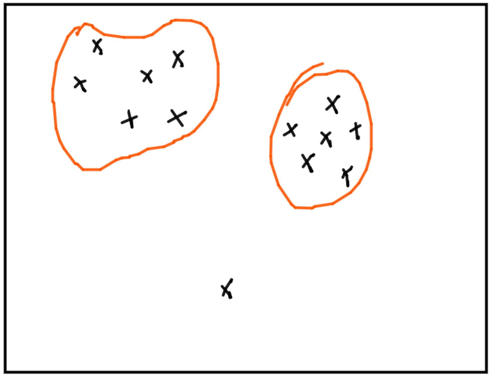 Représenter des données de manière pertinente.Exemple: les clusters pertinents sont ceux qui "amènent" le plus d’information.
Algorithmic Information Theory (AIT)
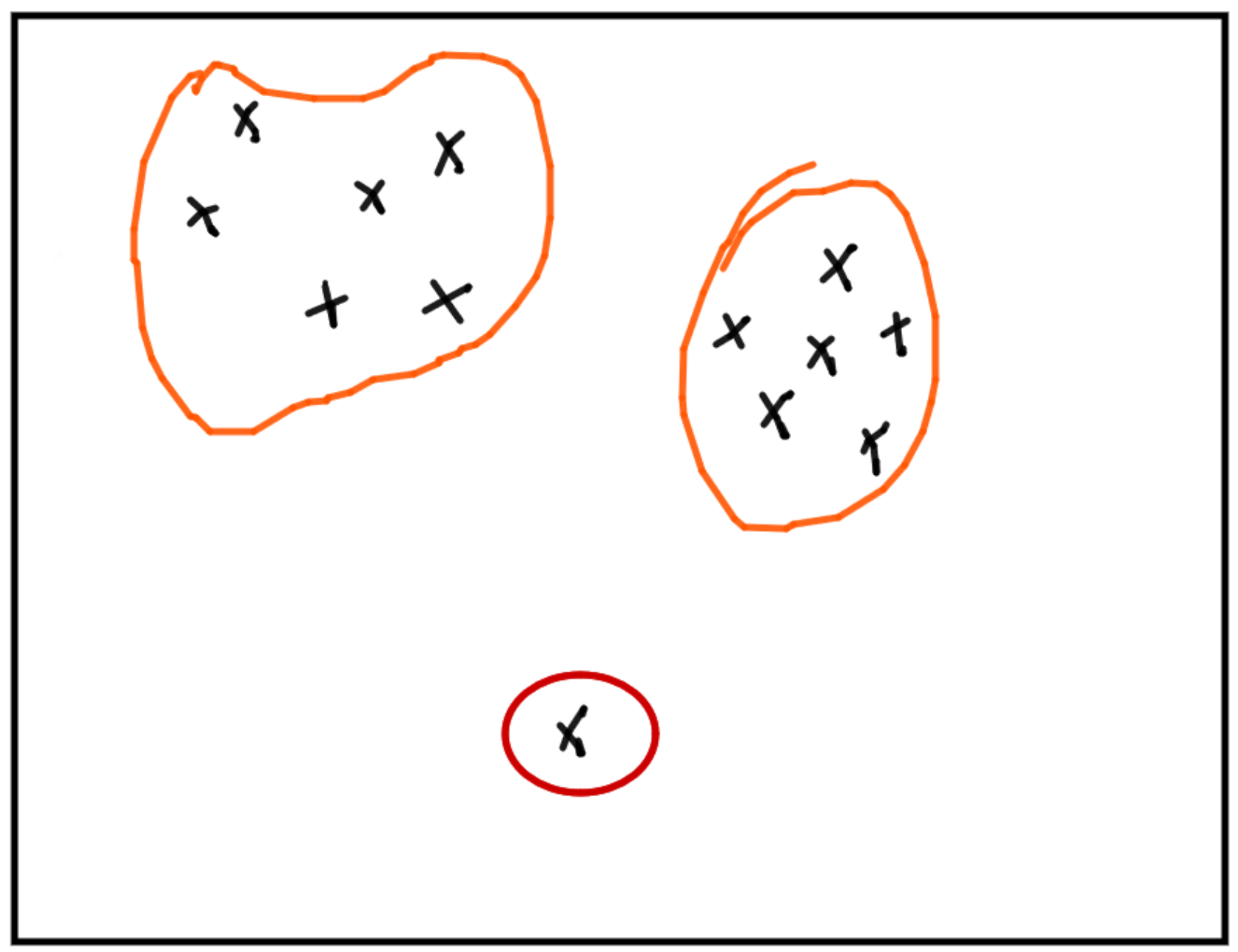 Représenter des données de manière pertinente.Un outlier est du bruit car il augmente artificiellement l’information
ou une anomalie car sa caractérisation demande peu d’information.
Algorithmic Information Theory (AIT)
Definition de l’information algorithmique:
Ray Solomonoff 1964, Andrei Kolmogorov 1965, Gregory Chaitin 1966 $$C(x) = min\{|p|; U(p) = x\}.$$ Taille du plus petit programme
qui engendre \(x\) sur la machine \(U\).
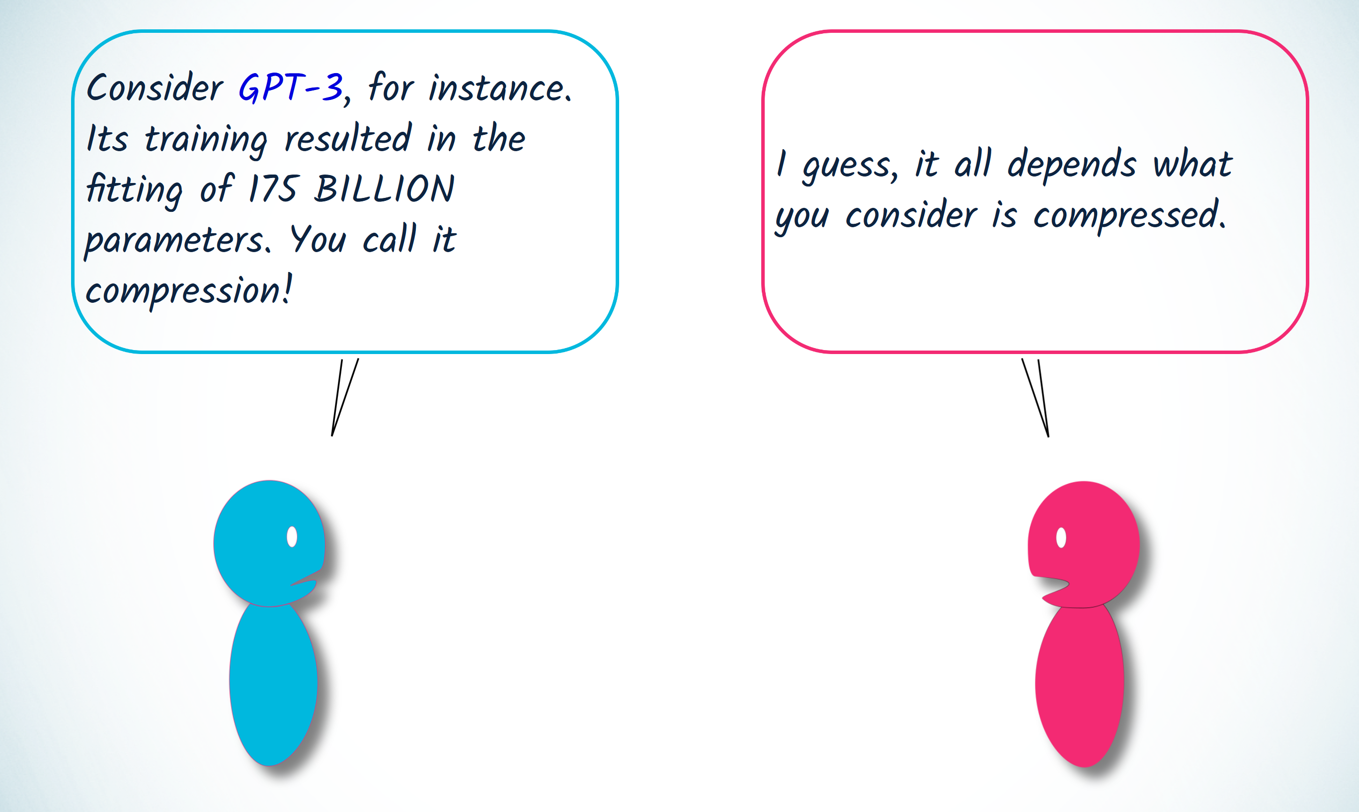
Thèse: La pertinence correspond à une baisse de complexité = compression
AIT & Machine learning
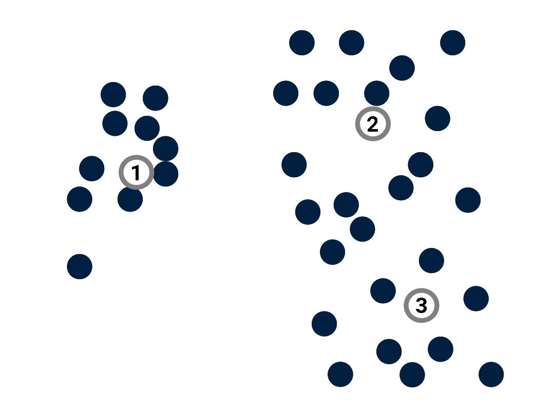
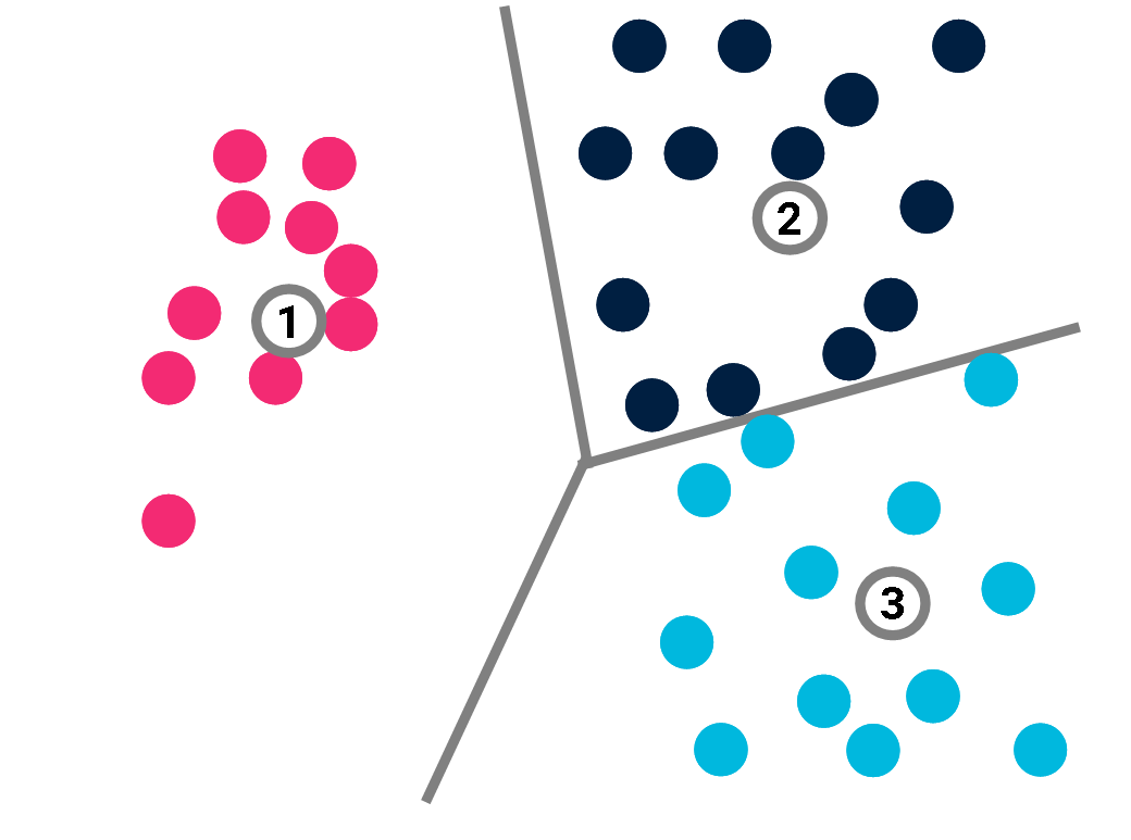
 Prototype-based models
A prototype is a point of the input space used to provide information about the distribution of data points.
Prototype-based models
A prototype is a point of the input space used to provide information about the distribution of data points. AIT & Machine learning
 Prototype-based models
A prototype is a point of the input space used to provide information about the distribution of data points.
Example: K-Means algorithm.
Prototype-based models
A prototype is a point of the input space used to provide information about the distribution of data points.
Example: K-Means algorithm. AIT & Machine learning
 Compression
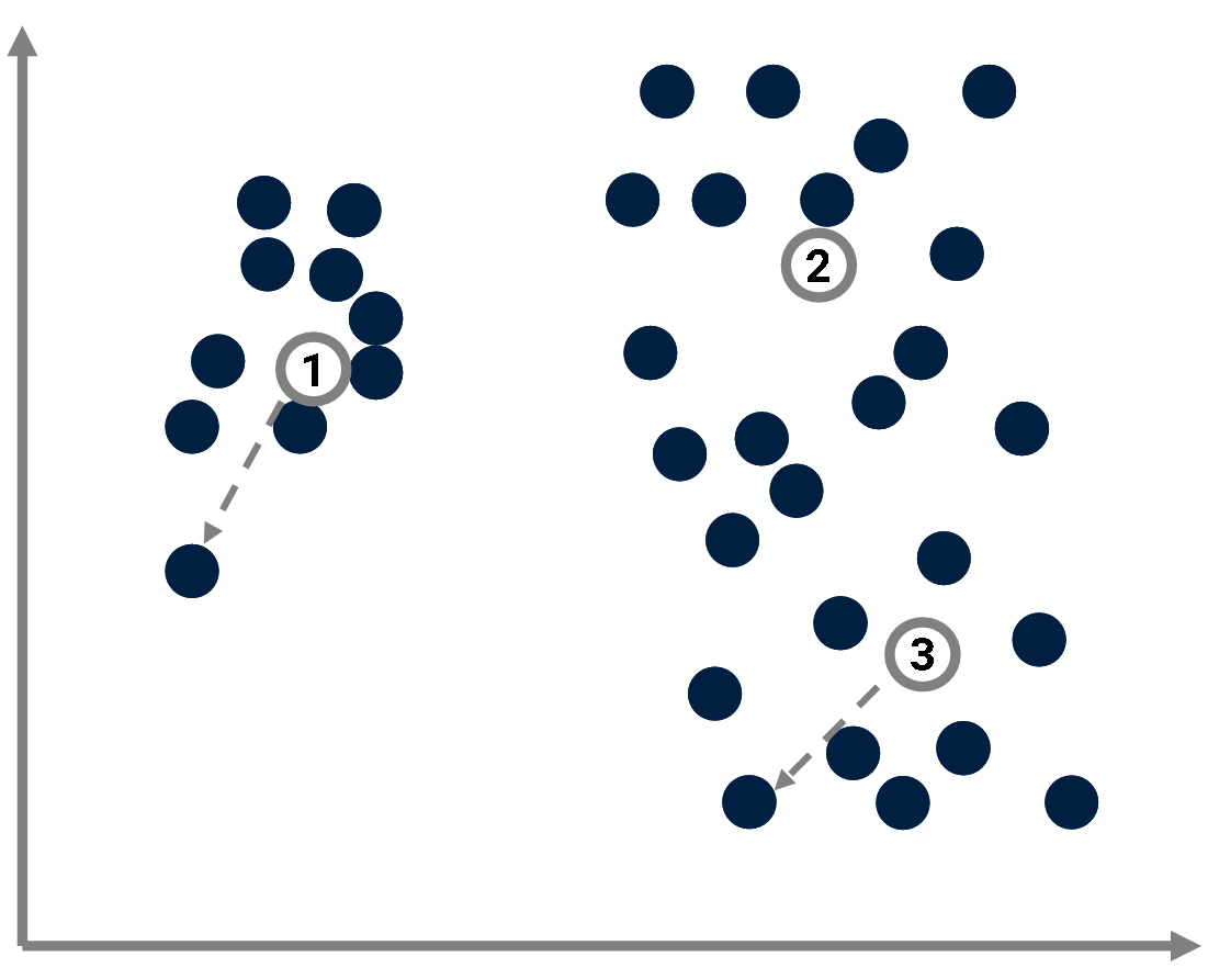
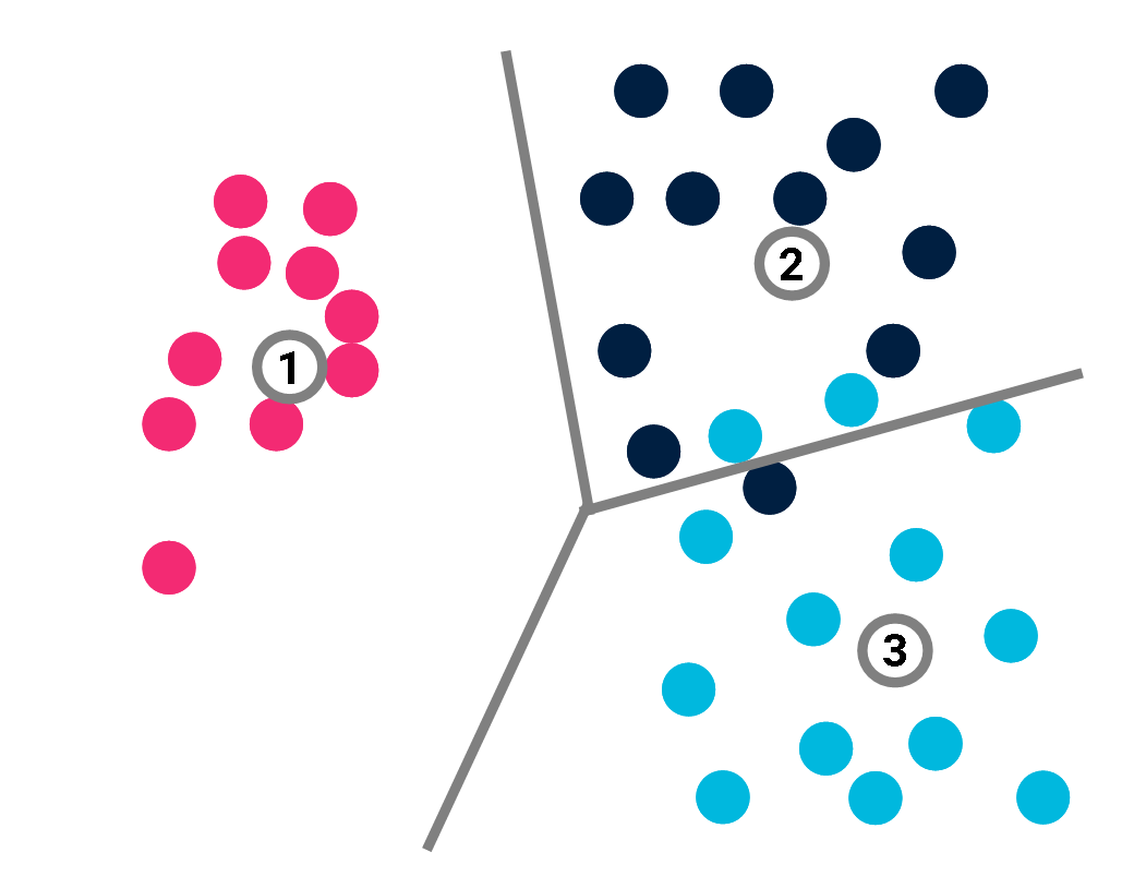
Prototype-based models can be seen as compression methods: Instead of describing data points by specifying their absolute coordinates,
Compression
Prototype-based models can be seen as compression methods: Instead of describing data points by specifying their absolute coordinates, AIT & Machine learning
 Compression
Prototype-based models can be seen as compression methods: Instead of describing data points by specifying their absolute coordinates,
Compression
Prototype-based models can be seen as compression methods: Instead of describing data points by specifying their absolute coordinates,
one considers their coordinates relative to the closest prototype.
AIT & Machine learning
 Compression
Prototype-based models can be seen as compression methods: Instead of describing data points by specifying their absolute coordinates,
Compression
Prototype-based models can be seen as compression methods: Instead of describing data points by specifying their absolute coordinates,
one considers their coordinates relative to the closest prototype. We get smaller numbers, hence the compression.
AIT & Machine learning
Compression
The complexity of a point \(x_j\) in the dataset \(X\) is bounded by the complexity of its coordinates \((x_{j_1}, \dotsc, x_{j_d})\):
$$ C(x_j) \leq C(x_{j_1}) + \dotsc + C(x_{j_d}),$$
where the complexity of coordinates depends on the precision \(\delta\) used to convert them into integers.
We get a "naive" upper bound of the complexity of the whole dataset \(X\): $$C(X) \leq \sum_j C(x_j).$$
AIT & Machine learning
Compression
If prototypes \(\{p_k\}\) are introduced,
the complexity of \(X\) is now:
$$ C(X) \leq \sum_k C(p_k) + \sum_i C(x_j|\{p_k\}),$$
where:
\(C(x_j|\{p_k\}) = \min_k C(x_j-p_k).\)
If the dataset exhibits some structure, suitable prototypes can be found and this estimate of \(C(X)\) will turn out to be significantly smaller that the "naive" one (hence the compression).
Conversely, and quite remarkably, this expression can be used to find the best prototype set \(\{p_k\}\)
(Cilibrasi & Vitányi, 2005).AIT & Machine learning
Compression
Prototypes \(\{p_k\}\) are relevant inasmuch as they lead to compression.AIT & Machine learning
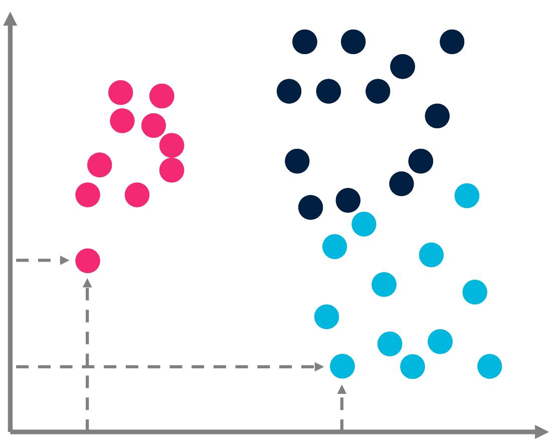
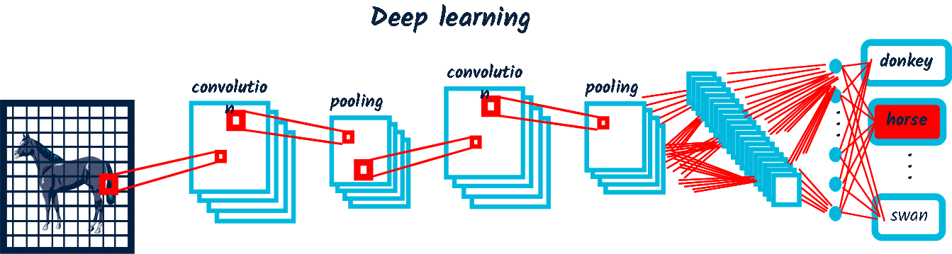
 Classification
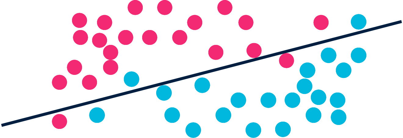
Now consider a classification task as an example of supervised learning.
Classification
Now consider a classification task as an example of supervised learning.
The problem is to associate a label (e.g. blue/red/dark) to each data point.
AIT & Machine learning
 Classification
Now consider a classification task as an example of supervised learning.
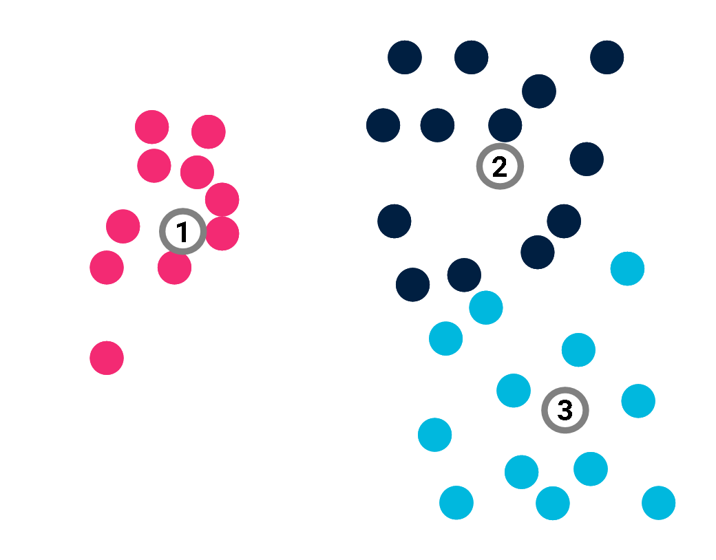
Classification
Now consider a classification task as an example of supervised learning.
The problem is to associate a label (e.g. blue/red/dark) to each data point. In doing so, they offer a compressed version of the classification.
AIT & Machine learning
 Classification
In a classification task, we consider a dataset \(X\) of \(|X|\) points \(x_j\). Each \(x_j\) is supposed to belong to a class labelled as \(y_j\). The problem is to learn which label \(y_j\) taken from the set of labels \(Y\) corresponds to \(x_j\).
The complexity of the classification is bounded by the amount of information required by rote learning.
$$C(\{(x_j, y_j)\} | X) \leq \sum_j C(\{y_j\}) \approx |X| \times \log(|Y|).$$
Classification
In a classification task, we consider a dataset \(X\) of \(|X|\) points \(x_j\). Each \(x_j\) is supposed to belong to a class labelled as \(y_j\). The problem is to learn which label \(y_j\) taken from the set of labels \(Y\) corresponds to \(x_j\).
The complexity of the classification is bounded by the amount of information required by rote learning.
$$C(\{(x_j, y_j)\} | X) \leq \sum_j C(\{y_j\}) \approx |X| \times \log(|Y|).$$AIT & Machine learning
 Classification
A prototype-based model \(\mathcal{M}\) would deduce the label of all points from those of its \(K\) prototypes \(\{p_k\}\), in the hope that:
$$\beta(x_i) = y_i.$$
Classification
A prototype-based model \(\mathcal{M}\) would deduce the label of all points from those of its \(K\) prototypes \(\{p_k\}\), in the hope that:
$$\beta(x_i) = y_i.$$AIT & Machine learning
 Classification
A prototype-based model \(\mathcal{M}\) would deduce the label of all points from those of its \(K\) prototypes \(\{p_k\}\), in the hope that:
$$\beta(x_i) = y_i.$$
The decision function \(\beta\) just returns the label of the closest prototype.
Classification
A prototype-based model \(\mathcal{M}\) would deduce the label of all points from those of its \(K\) prototypes \(\{p_k\}\), in the hope that:
$$\beta(x_i) = y_i.$$
The decision function \(\beta\) just returns the label of the closest prototype. AIT & Machine learning
Classification
The complexity of the model is given by the complexity of its prototypes and their labels:
$$C(\mathcal{M}) \leq \sum_k C(p_k) + K \times \log (|Y|).$$
Now:
$$C(\{(x_j, y_j)\} | X) \leq C(\mathcal{M}) + \sum_{j} {C((x_j, y_j) | X, \mathcal{M})}.$$
Since the decision function \(\beta\) is just a loop over the prototypes,
\(C((x_j, y_j) | X, \mathcal{M}) = 0\). So \(C(\{(x_j, y_j)\} | X)\) is found to be much smaller if \(K \ll |X|\) than if we only rely on rote learning. AIT & Machine learning
Classification
The complexity of the model is given by the complexity of its prototypes and their labels:
$$C(\mathcal{M}) \leq \sum_k C(p_k) + K \times \log (|Y|).$$
Now:
$$C(\{(x_j, y_j)\} | X) \leq C(\mathcal{M}) \ll |X| \times \log(|Y|).$$
We just have to remember the prototypes and their label to retrieve all labels, hence the compression.AIT & Machine learning
Classification
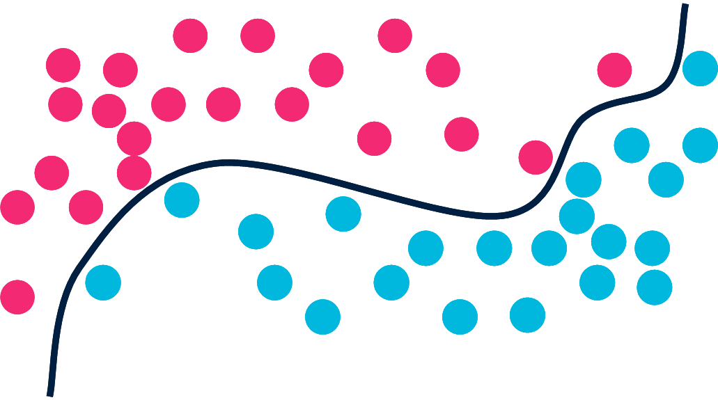
This is only true, however, if the model \(\mathcal{M}\) is perfect.AIT & Machine learning
 Classification
This is only true, however, if the model \(\mathcal{M}\) is perfect.If not:
\(C((x_j, y_j) | X, \mathcal{M}) \neq 0\).
For each misclassified point, we may just specify its index and the correct value of its label.
$$\sum_{j}{C((x_j, y_j) | X, \mathcal{M})} \leq \sum_{i=1}^{|X|} (C(i) + C(y_i)) \times \mathbb{I}(y_i \neq \beta(x_i)),$$
where \(\mathbb{I}\) is a function that converts a Boolean value into 0 or 1.
Classification
This is only true, however, if the model \(\mathcal{M}\) is perfect.If not:
\(C((x_j, y_j) | X, \mathcal{M}) \neq 0\).
For each misclassified point, we may just specify its index and the correct value of its label.
$$\sum_{j}{C((x_j, y_j) | X, \mathcal{M})} \leq \sum_{i=1}^{|X|} (C(i) + C(y_i)) \times \mathbb{I}(y_i \neq \beta(x_i)),$$
where \(\mathbb{I}\) is a function that converts a Boolean value into 0 or 1.AIT & Machine learning
Classification
This is only true, however, if the model \(\mathcal{M}\) is perfect.If not:
\(C((x_j, y_j) | X, \mathcal{M}) \neq 0\).More simply, if there are \(n\) misclassified points, we get:
$$\sum_{j}{C(\{(x_j, y_j)\} | X, \mathcal{M})} \leq n \times (\log(|X|) +\log(|Y|)).$$AIT & Machine learning
Classification To sum up:
$$C(\{(x_j, y_j)\} | X) \leq \sum_k C(p_k) + K \times \log (|Y|) + n \times (\log(|X|) +\log(|Y|)).$$
If \(n\) is small, this may still represent a huge compression as compared to rote learning.
The right-hand side of this inequality can be used as a loss-function to determine the best prototype-based classification.Minimum description length (MDL)

Minimum description length (MDL)
Minimum description length (MDL)
Minimum description length (MDL)
Machine learning: find a model \(\mathcal{M}\) to compress data \(\mathcal{D} = \{d_j\}\). $$C(\mathcal{D}) \le C(\mathcal{M}) + \sum_j{C(\mathcal{d_j} | \mathcal{M})}.$$ The most relevant model achieves the best tradeoff between its own complexity and the complexity of exceptions.
 We may then keep only the model
(= lossy compression if the model isn’t perfect)
to predict future data.
Vers un calcul de la pertinence
- Pertinence & Machine Learning
- Pertinence & AIQ (artificial IQ)
- Pertinence des événements
Artificial IQ
Artificial IQ
Artificial IQ
The most relevant answer achieves the greatest compression.$$n^{*n}$$
\(n\) repeated \(n\) times.
The most relevant answer minimizes the overall complexity of the sequence.
Artificial IQ

\(A\) → \(B\)
\(C\) → \(x\)
"\(A\) is to \(B\) as \(C\) is to \(x\)"
Doug Hofstadter is well-known for his original study of analogy. Let’s consider one of his favourite examples.
\(abc\) → \(abd\)
\(ppqqrr\) → \(x\)
Artificial IQ
\(abc\) → \(abd\)
\(ppqqrr\) → \(x\)
Most people would instantly answer
\(ppqqrr\) → \(ppqq\)\(ss\) Why should we consider it a more relevant solution than, say, \(ppqqrr\) → \(ppqqr\)\(d\)
Artificial IQ
\(abc\) → \(abd\)
\(ppqqrr\) → \(ppqq\)\(ss\)
\(ppqqrr\) → \(ppqqr\)\(d\) We have to compare two rules:
- increment the last item
- replace the last letter by d
Rule 2. has two drawbacks in terms of complexity:
- - it introduces a constant, d.
- - if we do not want to lose the structure of \(ppqqrr\), the rule should read:
"break the last item back into letters, and replace the last letter by d"
Artificial IQ
\(A\) → \(B\)
\(C\) → \(x\)
"\(A\) is to \(B\) as \(C\) is to \(x\)"
The most relevant answer minimizes the overall complexity.$$ x = argmin(C(A, B, C, x)).$$| Cornuéjols, A. (1996). Analogie, principe d’économie et complexité algorithmique. Actes des 11èmes Journées Françaises de l’Apprentissage. Sète, France. |
Artificial IQ
\(vita\) → \(x\)
Artificial IQ
\(vita\) → \(vita\)\(m\) Children learn their mother language from limited evidence. Analogy may play an important role. A system based on the complexity principle performed better than the state of the art on lexical analogies.
| Murena, P.-A., Al-Ghossein, M., Dessalles, J.-L. & Cornuéjols, A. (2020). Solving analogies on words based on minimal complexity transformation. International Joint Conference on Artificial Intelligence (IJCAI), 1848-1854. |
Vers un calcul de la pertinence
- Pertinence & Machine Learning
- Pertinence & AIQ (artificial IQ)
- Pertinence des événements
Relevance of events
- Personal news feed, chatbots
- Security (e.g. nuclear plant)
- Smart homes
- Diagnosis
- Abduction, CBR
- Anomaly detection
- Fraud detection
- . . .
Anomaly detection
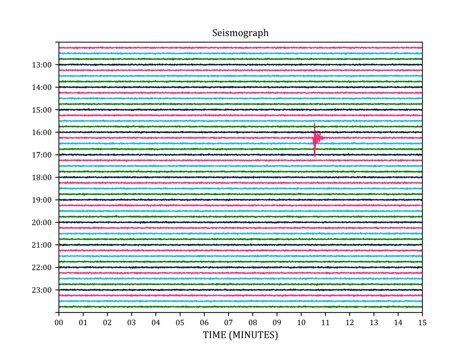
- outlier
Anomaly detection
- outlier
- impossibility
Anomaly detection

- outlier
- impossibility
- unanticipated events
Anomaly detection
- outlier
- impossibility
- unanticipated events
- coincidences
Anomaly detection
- outlier
- impossibility
- unanticipated events
- coincidences
Anomaly detection
- outlier
- impossibility
- unanticipated events
- coincidences
Anomaly detection
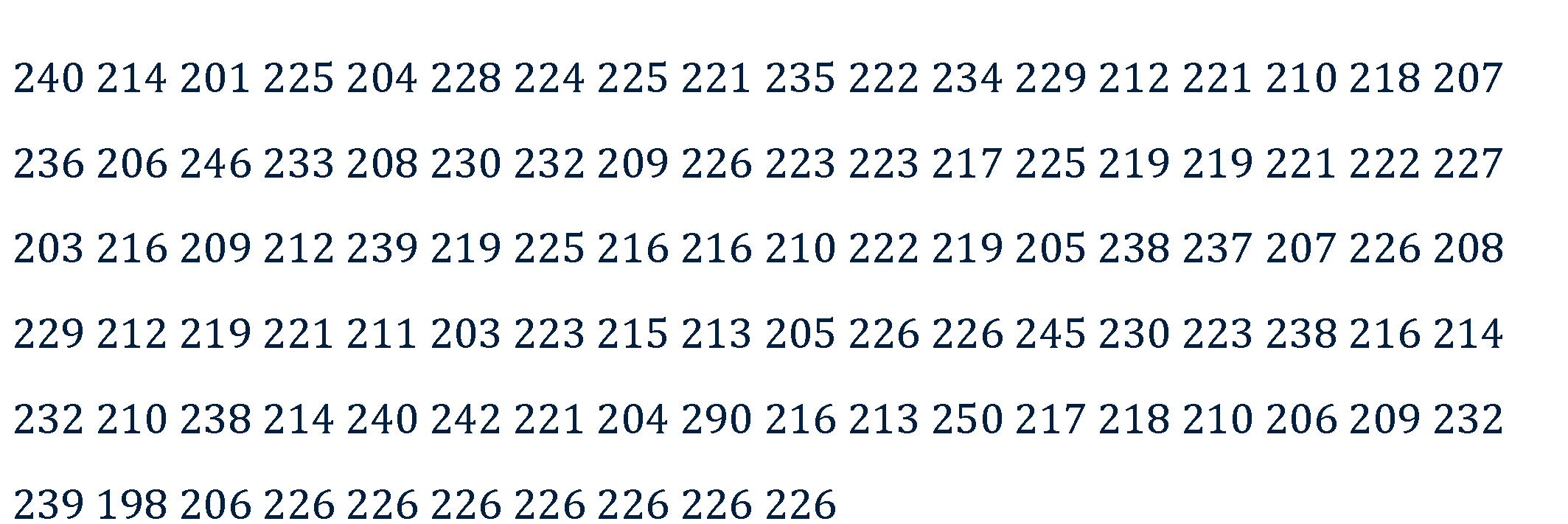
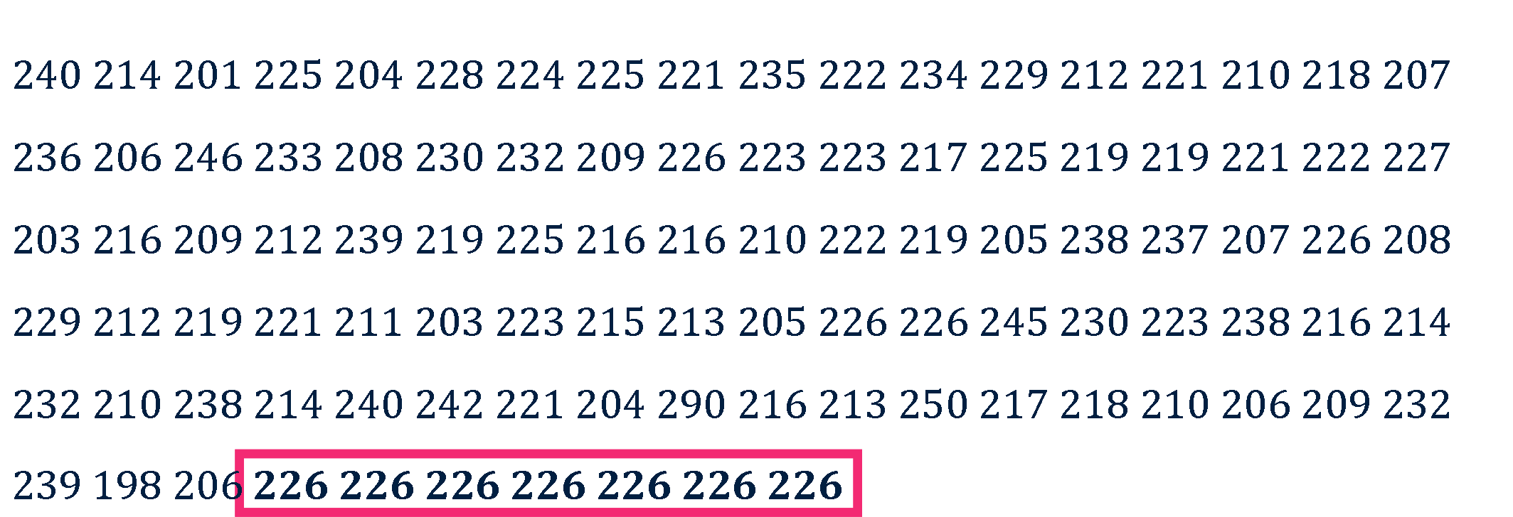
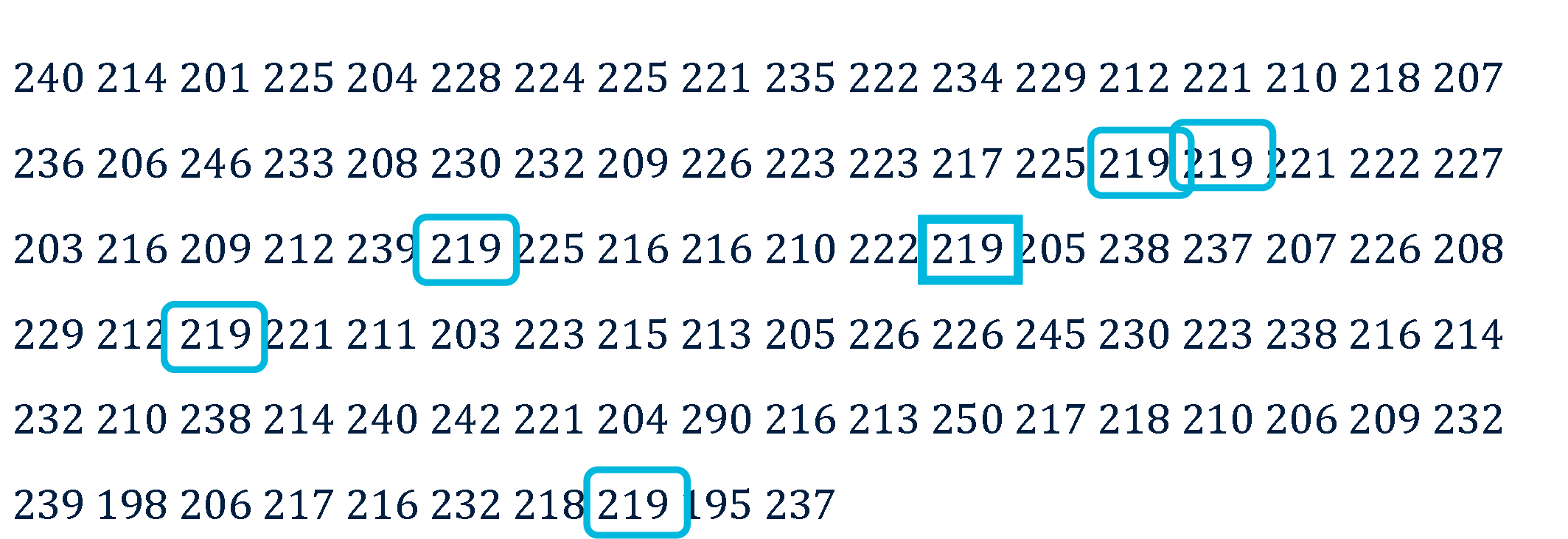
An anomaly is any event that is abnormally simple

Anomaly detection
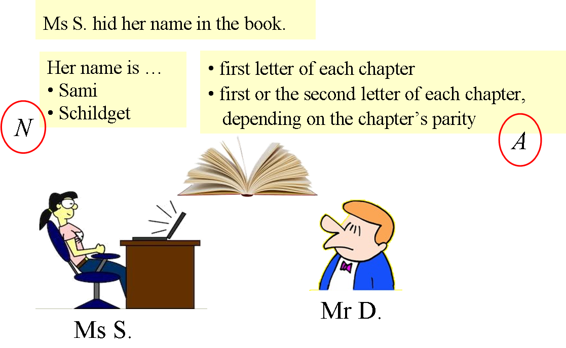
A Plagiarism story
$$ U = C(N) - C(A) $$
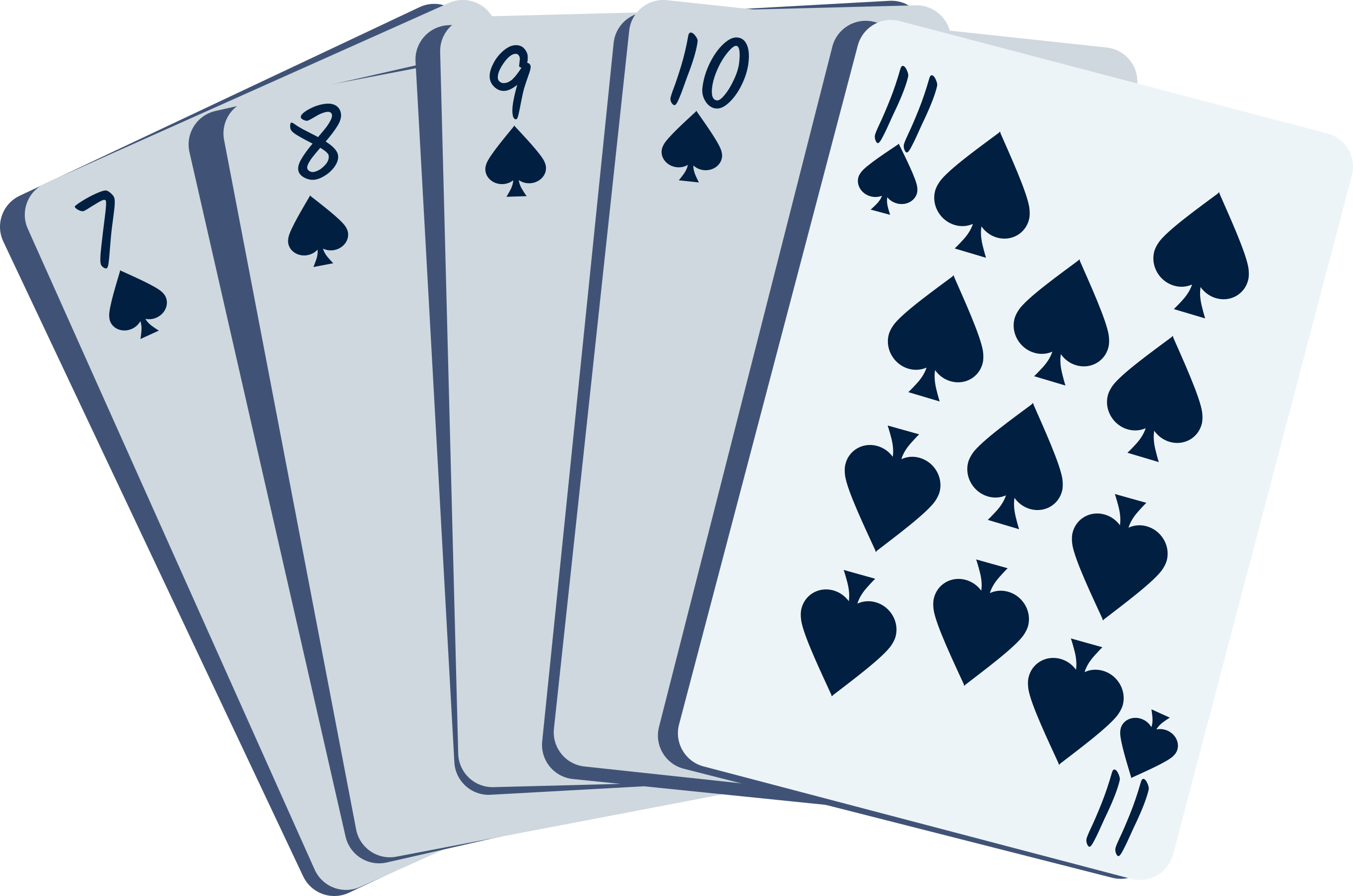
Unexpected events


Simple events seem unexpected, and thus relevant.
This effect can be quantified.
| Dessalles, J.-L. (2006). A structural model of intuitive probability.
ICCM-2006, 86-91. Trieste, IT: Edizioni Goliardiche. |
Unexpected events

Fortuitous encounter $$ U(s) = C(L) - C(p).$$
Subjective (im)probability
relevance = complexity drop
$$ p = 2^{-U} $$
$$ U(s) = C_w(s) - C(s) $$
Vers un calcul de la pertinence
- Pertinence & Machine Learning
- Pertinence & AIQ (artificial IQ)
- Pertinence des événements
- Pertinence des actions
Vers un calcul de la pertinence
Conclusion
La pertinence
- dans le cadre du machine learning
- dans le cadre d’une inducion (tests QI)
- pour les événements (anomalies, inattendu, ...)
- (et pour les actions)
(au sens de Kolmogorov).
relevance = complexity drop
Ce constat ouvre la voie à un calcul de la pertinence.Vers un calcul de la pertinence

- Deux livres
- Un MOOC sur l’information algorithmique
aiai.telecom-paris.fr - Un site Web
www.simplicitytheory.science
| Dessalles, J.-L. (2008). La pertinence et ses origines cognitives - Nouvelles théories. Paris: Hermes Science. |
| Dessalles, J.-L. (2019). Des intelligences très artificielles. Paris: Odile Jacob. |
| Dessalles, J.-L. (2013). Algorithmic simplicity and relevance. In Algorithmic probability and friends - LNAI 7070, 119-130. Springer. |