Objectives
The goal of this lab is to provide a gentle introduction to D3, a tool that is commonly used to create web-based, interactive data visualisations. After this lab, you should:
- Have a rudimentary understanding of web technologies: HTML, CSS, SVG, and JavaScript,
- Understand how to load data with D3 and bind them to their graphical marks, properties, and layouts,
- Know how to use D3 selections, scales, and axes.
What is D3?
D3 is a JavaScript library for creating Data-Driven Documents on the web. It is perhaps the most commonly-used environment for creating interactive visualizations on the web.
D3 simplifies many of the tasks of creating visualizations on the web. In order to use it, however, you will need to understand:
- JavaScript
- The HTML Document Object Model (DOM)
- The SVG vector graphics format
- Cascading Style Sheets (CSS)
In this lab, we will provide a brief introduction to these concepts so that we can create a basic visualization.
While it is not possible to master all of these concepts or even just the concepts of D3, this lab serves as a starting-off point. By the time you are finished, you should understand how to create a new D3 project from scratch, how to load data, and how to define a mapping from those data to visual objects on the screen. Moreover, you should have sufficient understanding of D3 to be able to read, understand, and adapt existing D3 examples to your own needs.
Getting started
You create a D3 visualization using any standard programming environment for web documents. You can use your own preferred environment for web development (e.g. TextMate, Sublime Text, vi, emacs, …), just make sure it has proper support for web development. If you’re not sure, here’s a link to Microsoft’s Visual Code editor.
Part 1
In this assignment, we are going to create a visualisation of places in France, with a basic representation and a smidgen (a chouia) of interactivity. You might end up with something like the following:
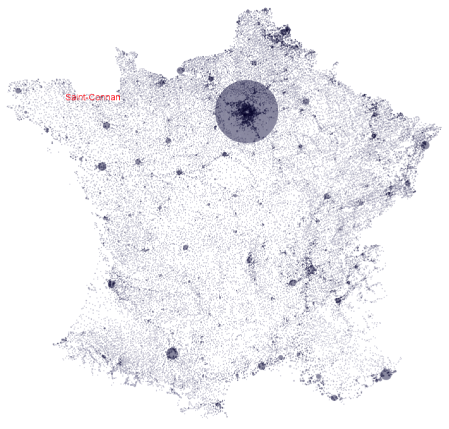
The data we will use comes from www.galichon.com/codesgeo. The original data was in the form:
- (name, postal code, insee code, longitude, latitude)
- (name, insee code, population, density)
To simplify things, we will instead use a pre-processed version of these data courtesy of Petra Isenberg, Jean-Daniel Fekete, Pierre Dragicevic and Frédéric Vernier. It merges these two datasets into:
- (postal code, x, y, insee code, place, population, density)
D3
D3’s name stands for Data-Driven Documents, and these documents use the web as their medium. That means that we have to think about two primary things: our data and our document. For our data, we need to:
- Load and parse the data,
- Choose an internal data structure to represent them.
For our document, we need to:
- Choose a representational structure,
- Define a mapping from the data to that structure.
Finally, web-based documents are not static pictures. We thus need to:
- Make the data interactive.
In general, we should follow « Shneiderman’s Mantra » : Overview first, zoom & filter, details on-demand. At minimum, we should let the user see the whole picture, dive in and focus on the parts of interest, and inspect the details of the data. We won’t quite do all of that in this assignment, but we should see the necessary pieces to put together.
Crash course on the Web for D3
D3’s medium is the web, which means that we will be working primarily with HTML, SVG, CSS, and JavaScript. HTML and SVG will describe the components to show in the visualisation, the CSS describes the various styling elements, and all of the code to load and store the raw data, as well as to connect them to the document will be in JavaScript. Let’s take a quick refresher of the basics of the web:
- HTML
- SVG
- CSS
- JavaScript
You can skip ahead if you’re already familiar with these technologies.
Crash course on HTML
A web page is generally written in HTML, which describes the contents of the web page to display. It consists of elements, described by tags. The first of these tags is the <html> tag, which tells the browser that this is an HTML document. All tags are written in angled brackets (<>). Most tags have a start tag and an end tag, where the end tag starts with a /. In our example, our document starts with <html> and ends with </html>. Everything between is considered as a child element of the <html> tag.
In this way, our web page defines a tree: the HTML document is the root of the tree. It contains two children: the <head>…</head> and the <body>…</body>. These elements, in turn, will contain their own children. The <head> describes meta-data about the web page, such as the <title> to display in the web browser, the character encoding (<meta charset="UTF-8">) so that accented characters appear correctly, or which scripts or style sheets to load.
In addition to having children, elements can also have attributes. We see an example of this in the meta tag above. It doesn’t have any children, but it does have one attribute, charset. An element may have zero or more attributes, separated by spaces and written in the form name="value".
Finally, some elements never have children, such as the meta tag we saw above or img, which loads an image into the document. These elements do not have a corresponding end tag, which is why we do not see </meta> above.
When the browser loads our HTML document, it creates the corresponding tree in memory. This tree is called the Document Object Model, or DOM. Our JavaScript code will interact with the DOM. That means that most of the time, we’ll refer to tags and attributes and children programmatically rather than writing angle brackets all the time.
There are a lot of different HTML tags, so you’ll probably want to keep a window open to the Mozilla Developer Network HTML Elements Reference. (If you use Duck Duck Go as your search engine, you may find !mdn and !mdnhtml useful.)
Crash course on SVG
There are two primary ways to draw directly to a web page: SVG and the HTML Canvas. While you can use the HTML canvas in D3, we’re going to use SVG, or Structured Vector Graphics.
SVG is a vector-based graphics format that uses an HTML-like syntax and can be embedded directly in an HTML document. Here’s an example:
<svg width="200" height="200">
  <rect x="10" y="10" width="125" height="125"
        style="fill: red; stroke: black; stroke-width: 2px;" />
  <rect x="40" y="40" width="125" height="125" rx="10"
        style="fill: blue; stroke: black; stroke-width: 2px; opacity: 0.7;" />
</svg>
In this example, we see a 200 × 200 pixel-wide SVG canvas with two rectangles in it. As you can see, their positions and dimensions are defined by their x, y, width, and height attributes. (The rx attribute gives the second rectangle rounded corners.) Their other properties are defined using CSS styles—via the style attribute. Note also that the <rect /> tags are self-terminating: they end with a /. This is a shortcut for immediately adding a closing tag: <rect /> thus is equivalent to <rect></rect>. In SVG, all tags must be closed.
There are several common shapes in SVG: <rect />, <circle />, <ellipse />, and <path /> are some of the more common ones. There is also a group element, <g> that can be used to group the other elements into layers on which you can, e.g., apply affine transforms. As always, the Mozilla’s developer documentation is a useful reference (!mdn or !mdnsvg in DuckDuckGo).
Crash course on CSS
We can use CSS to control the presentation, or style, of the various elements that we’ll be adding to our HTML document. This lets us control things like fonts for text, foreground and background colors, stroke and fill colors, or sizing and positioning of graphical objects. In the context of SVG, we can use CSS to control any of the properties of SVG elements (but not their attributes).
In CSS, we can define rules of the form property: value;. For example: color: red; or border: 1px solid steelblue; As you can see, some properties can have multiple values. These rules can be fairly complex, so you’ll probably want to keep a copy of Mozilla’s developer documentation open (or use !mdn or !mdncss on DuckDuckGo). Some common properties that we’ll use are color, background-color, fill, stroke, padding, opacity, and visibility.
We use CSS selectors to choose to which elements to apply the rules. CSS selectors can be fairly complex, but their basic components are tags, classes, and identifiers. For example, to make all <rect>s blue, you could use a rule:
rect {
    fill: blue;
}
To select all tags with the class map, you could select on .map. To select a tag with a specific id, say france, you would use #france. Finally, you can combine these in a lot of complex ways, such as:
svg.mapto select onlysvgtags with classmap:<svg class="map">.map rectto select only<rect>tags with a parent tag of class.map.
Given that, what might #france .map select?
Crash course on JavaScript
You already know how to program in Python or in Java, so you’ve already mastered the hard parts. JavaScript’s syntax falls roughly somewhere in between the two.
In JavaScript, you have to declare your variables, as in Java. On the other hand, you don’t need to specify their types, as in Python. Here’s an example :
let name = "Marie"; // Could also write as 'Marie';
let favoriteColor = 'red';
let favoriteNumber = 42;
const birthday = "17 March";
Note that we declare variables with let and constants with const.
In addition to strings and numbers, we can create lists, and dictionaries, just as in Python:
let colors = ["red", "orange", "mauve"];
let constants = { "pi": 3.14159,
                  "e": 2.7183,
                  "USS Enterprise": 1701 };
Dictionaries in JavaScript are actually objects, so you can use dot notation for any keys that are valide identifiers:
let area = constants.pi * r * r; // or we could have used the built-in Math.PI
let starshipRegistry = constants["USS Enterprise"];
We create a function with function:
function add2(n) {
    return n + 2;
}

// Or anonymously (like a lambda in Python)
let add3 = function(n) {
    return n + 3;
}
This latter form is common enough that there’s a shortcut syntax. We could have written the above as:
let add3 = (n) => { n + 3; }
There’s obviously a lot more to JavaScript, but that should be enough to get you up and running. As always, feel free to consult Mozilla’s developer documentation on JavaScript (you can use !mdn or !mdnjs on DuckDuckGo).
Creating our project
Let’s get back to our project.
First, let’s create a new folder for our project. Let’s call it France, and add three subfolders: css, js, and data. You should have a structure something like this:
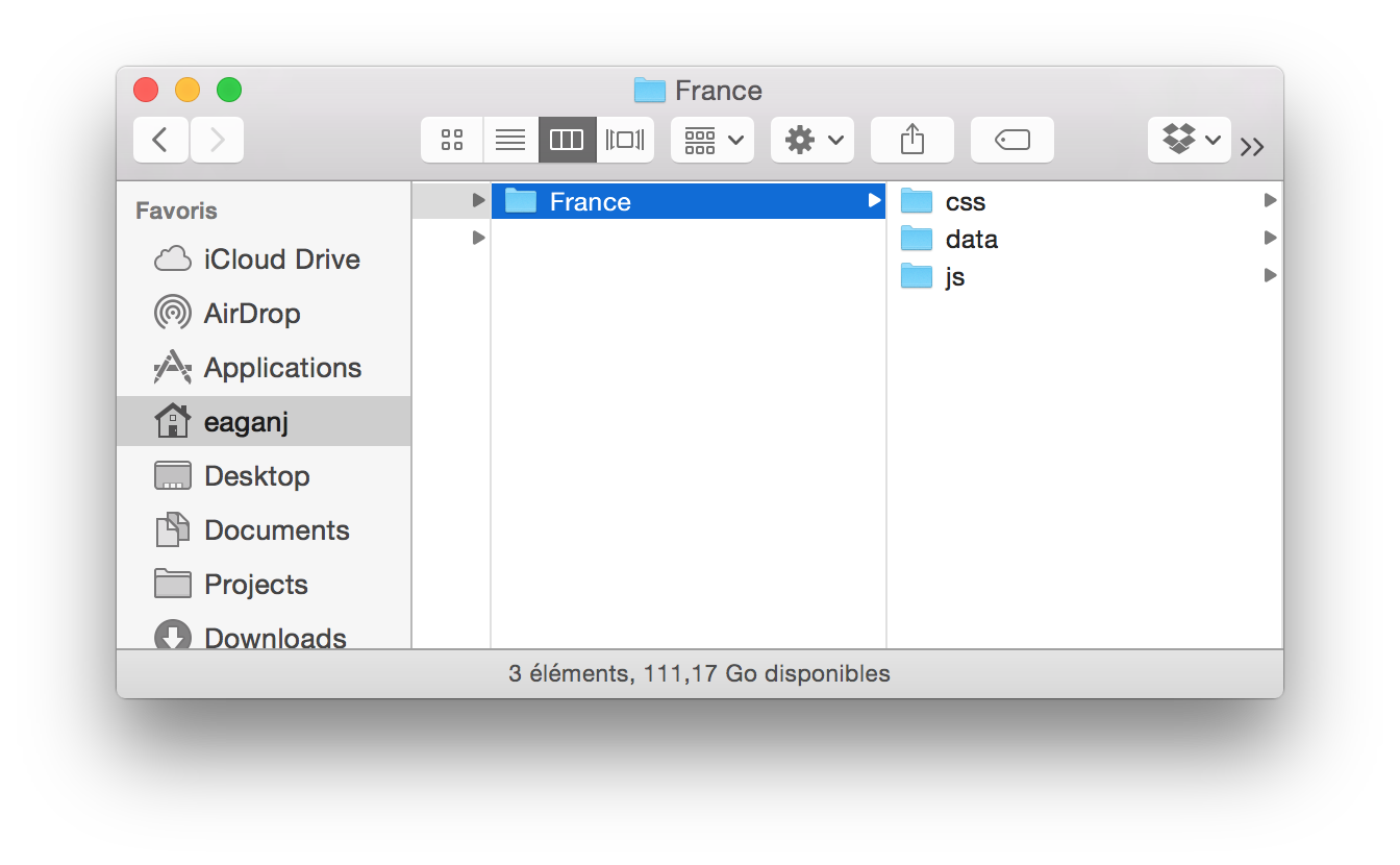
Our project will consist of four kinds of things:
- the data we want to visualize, which we will put in the
datafolder. - our D3 code, written in JavaScript, that will describe how to load and represent the data. We’ll put this in the
js(for JavaScript) folder. - style sheets to describe, e.g., the background color of our visualizations or how thick to make our bars in a bar chart.
- an HTML document that will link all of the above to create our visualization.
To work with this project, open it up in your favorite web programming editor. Notice that we have our three subfolders. The first thing we will need is a blank canvas to work with. In D3, our documents are “just” web pages. Create a new HTML document and add some boilerplate code for a basic HTML document. We’ll call this file index.html, which is the default web document that browsers will see when they open our project.
In this lab, I’ll start off by showing you the code to write. As we progress, I’ll show you less and less, and leave more open to your own interpretation. Please resist the temptation to just copy and paste the code. It’s important to understand what’s going on. Even if it seems obvious, writing (or typing) the code out by hand helps to reinforce things in your mind, so please type the following code in the window:
    <html>
    <head>
        <meta charset="utf-8">
        <title>Hello, France (D3)</title>
    </head>
    <body>
    </body>
    </html>
Let’s save this file as index.html. This gives us a blank web page with the title Hello, France (D3). Let’s make sure by opening it in our web browser. (In case you’re wondering about the <meta charset> line, that tells the web browser that our HTML uses UTF-8 text encoding, which helps make sure that our French accents will appear correctly on the screen.)
Let’s take a closer look at the document we just wrote above. If you’re already familiar with HTML and the DOM, feel free to skip to the next section, Loading D3.
Loading D3
This blank document is awfully boring, so let’s get ready to start adding some content to it. In D3, we will be adding our content programmatically, using JavaScript. To that, let’s add the D3 library to our project. Download the D3 library and extract it into the js/ folder in our project. Our project should now look like this:
- France
- css/
- data/
- index.html
- js/
- d3
- d3.js
- d3.min.js
- LICENSE
- d3
Let’s tell our project to use the d3.js library. Add the following line to the HTML header section of our document:
<script type="text/javascript" src="js/d3/d3.js"></script>
And now we need to create a file where we’ll put our own code. Create a new file, save it as js/hello-france.js, and tell our project to load it by adding the following like to the HTML body section of our document:
<script type="text/javascript" src="js/hello-france.js"></script>
Let’s make sure everything is loading correctly. Add the following line to the hello-france.js document:
alert("Hello, France!");
When we load our page, we should see our message in an alert box. If not, make sure you’ve correctly added your D3 <script> tag in your HTML header section and your hello-france <script> tag to the HTML body section.
If it’s still not working, let’s see if there’s anything else weird going on. Open your browser’s developer tools. In Chrome, go to Afficher > Options pour les développeurs > Outils de développement and click on the Console button. In Safari, open the preferences and go to the Avancées section. Make sure Afficher le menu Développement dans la barre des menus is checked. Then go to the menu Développement > Afficher le console JavaScript. If there are any errors in your code, they should appear here.
Most web browsers are very strict about JavaScript, even from local web pages. You may need to access your project through a web server. To do so, we will start a web server on the local machine using a builtin module of the python standard library. First, open a terminal/console window and cd to your project directory (France). Then run one of the following commands (depending on which version of python you have installed) to start a webserver on port 8080:
    python -m SimpleHTTPServer 8080
    python -m http.server 8080
You should then be able to access your project by going to http://localhost:8080. Warning: make sure that you run this command in your project directory, since it will give access to all of the files in the directory where you run it. If you run it from your home directory, any person on the internet could theoretically navigate to any file in your home directory. If you run it in the project directory, they can only access your project.
Congratulations! You now have a blank skeleton of your project set up. Once everything is in order, let’s go ahead and remove the alert() call, since that will get annoying quickly.
Creating an empty canvas
So far, we have an HTML document that loads D3 and our JavaScript code. We now need to create a drawing canvas we can use to create our visualization. To do that, we will use SVG, a vector graphics format that uses the same syntax as HTML. In fact, it is a superset of HTML and will be a part of our DOM. A blank SVG document, at its most simple, is just <svg></svg>. Let’s tell our hello-france.js to create a blank canvas for us, 600 pixels wide by 600 pixels high:
    const w = 600;
    const h = 600;

    //Create SVG element
    let svg = d3.select("body")
                .append("svg")
                    .attr("width", w)
                    .attr("height", h);
Let’s take a closer look at what this does. The first two lines should be straightforward: we create two global variables, w and h, that store the dimensions of our canvas. It’s the next part that is tricky. First, D3 creates a global variable, d3, that we will use to interact with the D3 system.
D3 uses a notion of selectors (similar to that of jQuery, if you’re familiar with it). As such, when we write d3.select("body"), d3 will traverse the DOM and return all of matching elements. In this case, all <body> elements. Our document (and any proper HTML document) only has one.
The next line, .append("svg"), appends a new <svg></svg> element as a child of the resulting <body> element. Thus, the DOM for a document with an empty body:
<body></body>
would become:
    <body>
        <svg></svg>
    </body>
Notice that we use a weird “chaining” syntax, where we write something like d3.select().append().attr().attr(). This works because the result of the .append() method is the newly added SVG element, to which we then set it’s “width” attribute to w (600) using the attr() method. D3 uses this “chaining” model for its methods, where methods that would otherwise be void instead return their object. Thus, the result of this .attr() is the SVG element whose attributes we are setting.
At the end of this, our document now looks like:
    <body>
        <svg width="600" height="600"></svg>
    </body>
If you look at your index.html file, you might think this is crazy, since it has not changed. There are no new lines in the file. Remember: in D3, we are programmatically modifying the DOM. When the web browser loads our document, it will create it’s internal model of the document (the DOM) using what was in the .html file. From then on, our JavaScript modifies this internal document. It is entirely ephemeral: it does not modify the .html file on disk.
{#
Side note: CSS classes
HTML and DOM elements can optionally have a class, which defines a type of element, or an id, which uniquely identifies a specific element. You could, for example, identify different SVG documents on the same web page by their class or id. You define a tag’s class with the the class attribute (e.g. <svg class="place-map"></svg>) or it’s id with the id attribute (e.g. <svg id="france-map"></svg>). You can also combine the two. Generally, if you are only going to have a single such element on the page, you would use an id. If you could potentially have multiple such elements, you would use a class.
We saw above that we could select on elements based on their tag. Thus d3.select("svg") would give us all <svg> elements in our document. You could also select on classes or ids. Thus d3.select(".place-map") would give us all elements with the class place-map, and d3.select("#france-map") would yield the element with the id france-map.
#}
Loading data
Now lets take a look at the data we’re going to use. Open them in your preferred text editor or in your favorite spreadsheet program. Notice that this a file containing a data table in a tab-separated format. What are the attributes of the data file? Do you notice anything interesting about the data?
The first thing we need to decide is how to store our data. Generally D3 stores data as a list of values. Here, each value will be a row in our table, which we will store as a JavaScript dictionary, or object. Each entry should have a postal code, INSEE code, place name, longitude, latitude, population, and population density. We will need to define a loader that will fetch each row of our TSV file and convert it into a JavaScript object.
Let’s go ahead and read the data into D3. D3 provides various importers to handle data in different formats, such as csv, tsv, json, etc. For more information, take a look at the D3 API. Since our data consists of tab-separated values, we are going to use the tsv loader.
What we want to do is write a function that loads the data from a file or URL, parses the data and stores it in memory, and then sets up the visualization. This is what we’re going to do, but we can’t do that all at once. What happens if the data file is really big, or if we’re loading it from a slow server? The interface would become unresponsive, or blocked, until it finished loading and processing all of that data.
Instead, D3 loaders generally run in the background. That means that our call to d3.tsv("data/france.tsv") will return immediately, before the data have finished loading. This is what is known as asynchronous or event-driven programming. We’re going to tell D3 to load our data, and then give it a function to call when it has finished. This will look something like
     d3.tsv("data/france.tsv")
       .get( (error, rows) => {
           // Handle error or set up visualization here
       });
The first line tells D3 that we want to load TSV data from data/france.tsv. The .get() method tells it to start loading and that, when it is done, it should call a function. That function has two parameters, error, and rows. This code in our function is not executed right now, but it will be at some point in the future.
If you’re curious about what’s going on here, we’re creating an anonymous function and using it at a parameter to the .get() method. When the get() method finished loading its data in the background, it will then call this anonymous function.
Let’s go ahead and add this loader to our hello-france.js:
     d3.tsv("data/france.tsv")
       .get( (error, rows) => {
            console.log("Loaded " + rows.length + " rows");
            if (rows.length > 0) {
                console.log("First row: ", rows[0])
                console.log("Last  row: ", rows[rows.length-1])
            }
       });
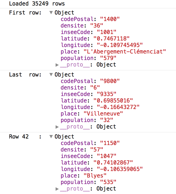
Reload the page to run the code. Here, we’re just outputting some debugging information to the console, so we can make sure everything is loading correctly. Take a look at the first and last rows. Maybe try with a few random rows, too, just to do a spot-check. Does everything look right?
Converting the data
So far, everything looks pretty good, but you might have noticed a problem at the end of the previous section. If we take a closer look at our console log, we should see something like this:
Do you see the problem?
It’s subtle, but it’s there.
Try to see if you can figure it out before you read on.
Did you figure it out?
Yes, that’s right, all of our values are strings, including numerical attributes such as population, longitude, and latitude. Thankfully, there’s a concise way to convert these strings to numerical values in JavaScript: use the + operator, as in let populationAsNumber = +populationAsString;.
We just need a way to tell D3 to apply our conversions to each row that it loads. Not surprisingly, D3 loaders have a method to do this called row(). The row() method takes a function as a parameter and returns the loaded row. This function takes two parameters:
d, a datum, as a JavaScript dictionary whose keys are the column labels from our TSV file, andi, the index of the current row.
Let’s update our loader to clean up these rows as they load:
    d3.tsv("data/france.tsv")
      .row( (d, i) => {
            return {
                codePostal: +d["Postal Code"],
                inseeCode: +d.inseecode,
                place: d.place,
                longitude: +d.x,
                latitude: +d.y,
                population: +d.population,
                density: +d.density
            };
      })
      .get(/* this code unchanged from before */
      );
Notice that the first column has a space in its name, and is thus not a valid JavaScript attribute name. We therefore need to access it using dictionary notation: d["Postal Code"]. The others are valid attribute names, so we can just access them as attributes, as in d.place. Both are equivalent. Notice also that we use the dictionary key postalCode instead of “Postal Code”. That way, we can more easily access our post-processed data rows as d.postalCode instead of d["Postal Code"].
Try reloading the page in your browser and make sure you see the right thing on the console.
Drawing
Hooray, we now have a way to get data into our document, and we’ve seen how we can create our own internal data model. So far, it doesn’t really do us much good if we can’t somehow draw it to the screen. Let’s figure out how to do that.
First, we’re going to need to make sure we save the data somewhere we can use it. The rows parameter to our get() method has the data, so we just need to save it somewhere accessible from the rest of our program. Add a new global variable, just after your w and h variables, to store the dataset. Let’s call it dataset:
    const w = 600;
    const h = 600;
    let dataset = [];
Now, at the end of the .get() method, store our rows in this variable: dataset = rows;. Then add a call to draw(), which we’ll define shortly. That way, once all of the data has been loaded, we will call draw() to draw all the data.
Enter, update, exit
Now we get to the hardest part of D3: enter, update, exit. D3’s data model takes some getting used to. What we’re really doing is defining rules that will be executed whenever our data changes in some way:
enterwhenever a new data entry is created,updatewhen a value changes, andexitwhen a value is deleted.
Each of these rules will tell D3 what to do, such as creating or removing a (new) element on our canvas or updating certain attributes of our elements.
In this example, our data set is not going to change, so we only need to use enter. For dynamic data sets, where entries may be created or removed while the page is being shown, or where entries may change values, you will need to use update and exit as well.
Let’s just create a small rectangle for each place in our data set:
    function draw() {
        svg.selectAll("rect")
            .data(dataset)
            .enter()
            .append("rect")
    }
So far, this function won’t actually draw anything, because we have not yet told it how to connect our rectangles to the data. We’ll do that shortly, but first let’s try to understand what’s going on above, since it’s a bit strange.
First, we use the svg variable we created earlier, which represents our canvas. We tell it to select all of the <rect>s in our drawing, then tell it to bind them to the data we stored in our dataset variable. We then use .enter() to specify that, when new data comes in (such as when we first load the document), it should append a new <rect> element to our canvas.
If your brain is having a hard time digesting this, that’s ok. It feels as if we’re eating our cake and then baking it, yet somehow we manage to eat a fully-baked cake. Is looks as if we first select all of the rects, then we create them. This is where we need to remember that what we are doing is defining a set of rules that will be used. Thus, we are not actually selecting all of the rects in the svg canvas. Instead, we are defining a rule that will be applied to all rects. When a new entry is created in our dataset, the rules we specify here after .enter() will be applied to them, which in this case is to create a <rect>, which is how SVG describes rectangles. (We could also specify .update() and .exit() rules that will be used when rows are modified or removed from our data set.)
When we create a new rectangle, we want, for now at least, it’s size to be 1 × 1 pixels. We do that by specifying SVG and CSS attributes for the rect:
    function draw() {
        svg.selectAll("rect")
            .data(dataset)
            .enter()
            .append("rect")
            .attr("width", 1)
            .attr("height", 1)
            // ...
    }
We also want its position to correspond to its longitude and latitude. That’s a little bit trickier. So far, the width and height have been constant (1), but the position will be a function of the data (it’s longitude and latitude). We need a way to specify a different value specific to each point.
In D3, we can do that by passing in a function as the value. The function takes a single value as a parameter: our data point. It returns the value that we want to use. Thus, we can replace the ellipsis in the above code with:
    .attr("x", (d) => d.longitude)
    .attr("y", (d) => d.latitude)
What do you expect to happen when you run the program? Try it out. Reload the page. What actually happens? Can you think of a reason why we don’t see anything on the screen?
Before you get too far trying to figure out why you don’t see France, take a closer look at the top, left of our document. It’s subtle, but we do have a bunch of rectangles being created. Try to think about what might be going on.
Still not sure? Let’s take a closer look at our data. Recall that each row is in the following format:
(postal code, x, y, insee code, place, population, density)
We only use the x and y columns. Think about it before continuing on.
Data scales
The x and y columns in the data set are expressed in longitude and latitude, not in terms of pixel coordinates on the screen. All of our coordinates correspond to a single pixel, which is being clipped to the top left of our canvas since all of France has a negative longitude.
We need to create a mapping from longitude, latitude to x, y-coordinates on the screen. Assuming a flat projection, the math is actually pretty simple. Since this kind of problem is very common, D3 has a builtin concept for this: scales. We can define scaling functions that will map a value from one coordinate space to another. Here, we just have a linear scaling function, so we can use D3’s linear scales:
d3.scaleLinear()
To do so, we will need to create our x-scale and y-scale that will map a longitude, latitude onto our 600 × 600 pixel canvas. To do that, we need to set the scale’s domain and range, which correspond to the potential values that an input can take, and the range of values an output can take on.
We could take a look at our input and figure out our domain from the longitudes and latitudes of our data set, but instead we’ll compute it dynamically from the data set. That way, if some day we want to show places in the United States or China or Mars, our visualization would handle it without trouble. To do so, we use D3’s extent() function, which calculates the extent of the data set: the range of a given column’s min and max values. We will store these scales in two global variables: x and y. Go ahead and add these to the top of our file.
Now modify our data loader to compute the scales when the data is finished loading:
    x = d3.scaleLinear()
        .domain(d3.extent(rows, (row) =>  row.longitude;))
        .range([0, w]);

    y = d3.scaleLinear()
        .domain(d3.extent(rows, (row) => row.latitude))
        .range([0, h]);
These scales will take a value in a given domain and normalize it to the given range. Let’s modify our drawing loop to use them as follows:
    .attr("x", (d) => x(d.longitude) )
    .attr("y", (d) => y(d.latitude) )
Let’s try running the program one more time, and this time we should be able to marvel in the wonder of your beautiful drawing. Or fix any bugs and then marvel.
Graphics coordinates
Have you noticed something peculiar about our map of France?
In most graphics environments, the origin (0, 0) is located at the top, left of the canvas. Latitudes, on the other hand, start at the equator, which we tend to think of as being to the bottom of France. No worries, all we need to do is invert either our domain or our range in the above mapping function.
Make that change and re-run the program. Is Corsica at the top or the bottom? Do we indeed see the Finistère next to the Channel, or is it hanging out in the Mediterranean?
On your own…
That’s great for getting started, but what we’ve created so far is really only little more than an info vis “Hello, world” (or, more properly, “Hello, France!”).
To better understand our toolbox, let’s look at the D3 API reference. These are the builtin methods and functions of D3. (There’s a new version of D3 that recently came out. This tutorial uses version 4.) There’s a lot to take a look at. You may also wish to learn more about CSS or SVG.
You should now have the tools you need to update your visualization to:
- Show population and density
You’re also going to make your visualisation interactive. When the user clicks on a place, draw its name and postal code. You will need the following tools to do so:
Text rendering
Add a new text item below your canvas that you will use to display the names of places as the user hovers over them.
User events
You can use D3’s .on() method to add callbacks for certain events, such as mouseover or mouseout when the user hovers or unhovers on an item. For example:
.on("mouseover", function(d) { /* ... */ })
 Assignment based on one by Petra Isenberg, Jean-Daniel Fekete, Pierre Dragicevic and Frédéric Vernier under a Creative Commons Attribution-ShareAlike 3.0 License.